Components in Forecasting
Forecasting deals with the analysis and detection of trends in the time-series data. The components of forecasting are,
- Data Exploration: Data Exploration is used to explore the time-series data. It helps in identifying the underlying parameters required for forecast model building.
- Modeling: Modeling is used to drag-and-drop the forecasting algorithms in the workbook for analysis. Rubiscape provides the following algorithms in Forecasting.
- Autoregressive Integrated Moving Average (ARIMA)
- Auto ARIMA
- Automated Exponential Smoothing
- Holt Exponential Smoothing
- Holt-Winters Exponential Smoothing
- LSTM
- Moving Average
- Random Walk
- Seasonal Autoregressive Integrated Moving Average (SARIMA)
- Simple Exponential Smoothing
- Data Preparation: Data Preparation is used to perform a variety of data preprocessing tasks. The following functionalities are present in Forecasting under Data Preparation.
- Data Preparation (tasks such as data aggregation, missing value imputation, and data transformation using mathematical measures and functions on the time-series data.)
- Lags (a feature engineering technique used in time-series analytics to predict values for a given set of data)
- Train-Test Split (splitting of data and tagging the records into training and testing data)
Using Data Exploration
In Forecasting, Data Exploration is used to explore time-series data and plot the variations and trends. It identifies the underlying parameters to build forecasting models.
To use Data Exploration, follow the steps given below.
- Open a workbook that you want to edit. Refer to Opening a Workbook.
- Drag and drop a dataset from Connect (in the task pane) on the Workbook canvas.
- Click on the Dataset node and select the required Data Fields in the Properties pane.
- Validate the node and click Save.
- Click Run in the function pane. The node is successfully run, and a green tick mark appears.
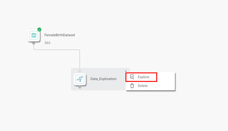
- Drag and drop the Data Exploration node from Forecasting (in the task pane) on the Workbook canvas.
- Connect Data Exploration to the Dataset node.
- Click the Data Exploration node and select the corresponding parameters from the Properties pane.
- Click the Data Exploration node again.
- Click the vertical ellipsis (
 ) in the top-right corner of the node.
 - Click Explore.
Notes: |
|

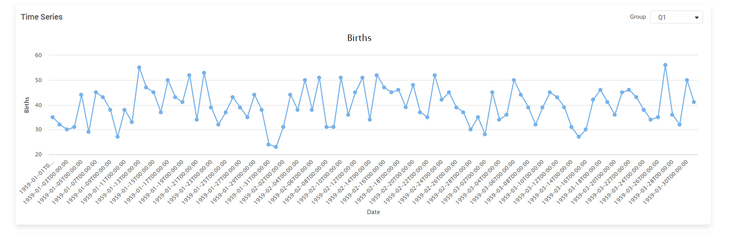
The output of the Data Exploration node is displayed. The Result page shows a set of charts, some test plots, and corresponding statistical parameters for time-series data.
Understanding the Data Exploration Result Page
On the Data Exploration Result page, you see a set of charts and some test plots, and corresponding statistical parameters. These are listed below.
- Time-series charts
- Time Series plot
- Trend plot
- Seasonality plot
- Irregularity plot
- Test plots and statistical parameters
- ACF plot
- PACF plot
- Ljung Box plot
- DF Test
Time-series charts
The time series chart displayed on the Result page is given below. It shows the variation in the target variable concerning time for the selected Group variable.
Here, the chart shows the variation in Births with Date for Group Q1. You can select groups using the drop-down and plot corresponding charts.
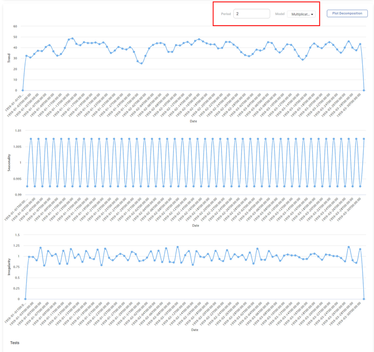
Apart from the time-series chart, the page also displays charts for other time-series components. For this, a technique called Decomposition is used. It separates (decomposes) the historical data into its components and then uses them to create a forecast. This technique is comparatively accurate than a simple time-series plotline.
The plots corresponding to Decomposition are collectively called the Decomposition plots. These are
- Trend (Trend component)
- Seasonality (Seasonal component)
- Irregularity (Noise component)
For plotting the Decomposition charts, you should select
- a specific period for which prediction is to be done and
- the model (additive or multiplicative); you can plot the three decomposition plots for the selected Group.
For example, in the figure below, you see the decomposition plots for a Multiplicative model and period equal to two (2).
Note: |
|
Test Plots and Statistical Parameters
The test plots and statistical parameters are given below.
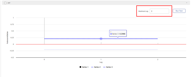
ACF Plot
It is the graph between the autocorrelation function of any series and its lagged values. ACF considers all components of the time series (trend, seasonal, cyclic, and residual) while determining the correlation. Hence it is also called the Complete Auto-Correlation plot.
The figure below displays an ACF plot for a Maximum Lag value of 2.
PACF Plot
It is the graph between the partial autocorrelation function of any series and its lagged values. PACF finds the correlation of the residual component of the time-series with its next lagged values. Thus, earlier determined correlations are removed before finding the next correlation.
The figure below displays a PACF plot for a Maximum Lag value of 2.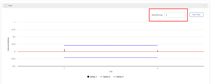
Ljung Box Test
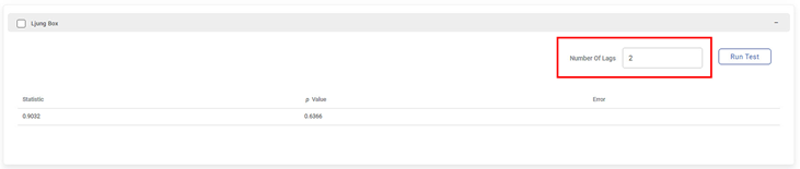
The Ljung Box test is a statistical test that detects the absence of serial autocorrelation, determined up to a specific lag value. It determines whether the autocorrelations for errors (residuals) are non-zero. The Ljung Box test is a test to detect a lack of fit. Models are understood to be showing no noticeable lack of fit if the residual autocorrelations are small.
The figure below shows the displayed Ljung Box test parameters for the Number Of Lags two (2). You get the Ljung Box test statistic, p value, and the error.
DF Test
The augmented Dickey-Fuller test is used to verify the null hypothesis that a unit root is present in a time-series sample. A unit root is some random process feature that can cause issues with statistical inferences in time-series models.
The Augmented DF test statistic is a negative real number. The more negative the statistic more likely is the rejection of the null hypothesis that a unit root is present for some confidence level.
The figure below shows the displayed DF test parameters for the Number Of Lags equal to two (2). You get the DF test statistic (a negative number), p value, and the error.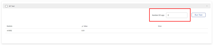
Note: |
|
Using Data Preparation
In Forecasting, Data Preparation is used to perform a variety of data preprocessing tasks on the time series data.
It contains the following functionalities.
- Data Preparation
- Lag
- Train-Test Split
To use Data Preparation, follow the steps given below.
- Perform steps 1 to 5 of Using Data Exploration.
- Drag and drop the Data Preparation node from the Data Preparation menu in Forecasting (in the task pane) on the Workbook canvas.
- Connect the Data Preparation node to the Dataset node.
- Click the Data Preparation node and select the corresponding parameters from the Properties pane.
- Click the Data Preparation node again.
- Click the vertical ellipsis (
 ) in the top-right corner of the node.
 - Click Run from the drop-down.
The node is successfully run, and a green tick mark appears. - Click the Data Preparation node again and click the vertical ellipsis.
- Click Explore from the drop-down.

The output of the Data Preparation node is displayed. The Result page shows the following plots related to the time-series data.
- Accumulation
- Missing Value Imputation
- Transformation
- Differencing
The output also displays the Trace. In this case, the Trace tab shows the user a list of tests that were run.
Refer to Time-Series Data Preparation in Forecasting in the Algorithm Reference Guide.
Related Articles
Working with Forecasting
What is Forecasting Forecasting is an integrated tool to streamline and automate the forecasting process. With Forecasting, one can efficiently explore and analyze large volumes of time-series data without manually coding models.Creating a Workbook in Forecasting
To create a workbook, follow the steps given below. On the home page, click the Create icon (). Hover over the Forecasting tile and click the Create Workbook button. Create Workbook screen is displayed. Enter the Name for your workbook. Enter the ...Building Algorithm Flow in a Forecasting Workbook Canvas
Building algorithm flow in a Forecasting Workbook is similar to that in Model Studio. To build algorithm flow in a Workbook Canvas in Model Studio, refer to Building Algorithm Flow in a Workbook Canvas.Holt Exponential Smoothing
Holt Exponential Smoothing is located under Forecasting > Modeling > Holt Exponential Smoothing. Double-click or drag-and-drop the algorithm to use in the workbook canvas. Click the algorithm to view and select the different properties for analysis. ...Deleting a Workbook in Forecasting
Deleting a Workbook To delete a workbook, follow the steps given below. On the home page, click Workbooks. Recent Workbooks for the selected workspace are displayed. Hover over the workbook you want to delete, click the vertical ellipsis, and click ...