Gradient Boosting in Classification
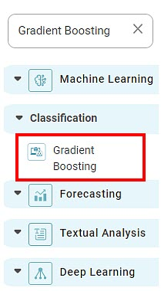
The category Gradient Boosting is located under Machine Learning in Classification on the feature studio. Alternatively, use the search bar to find the Gradient Boosting test feature. Use the drag-and-drop method or double-click to use the algorithm in the canvas. Click the algorithm to view and select different properties for analysis.
Gradient Boosting is a robust machine learning algorithm in the ensemble learning family. It integrates several weak predictive models, often decision trees, to produce a powerful predictive model. For problems involving classification and regression, Gradient boosting is highly successful.
The "Gradient" in Gradient boosting uses Gradient descent optimization to minimize the loss function. In each iteration, the algorithm calculates the negative Gradient of the loss function concerning the predicted values. This Gradient represents the direction in which the loss function decreases the fastest. The weak model is then trained to expect this Gradient, and the resulting predictions are added to the ensemble.
The boosting aspect of Gradient boosting comes from the fact that the weak models are combined sequentially. Each new model is trained with a focus on improving the ensemble's performance by targeting instances that were previously poorly predicted. The predictions from all weak models are combined using a weighted sum. The weights assigned to each model are typically determined based on their performance.
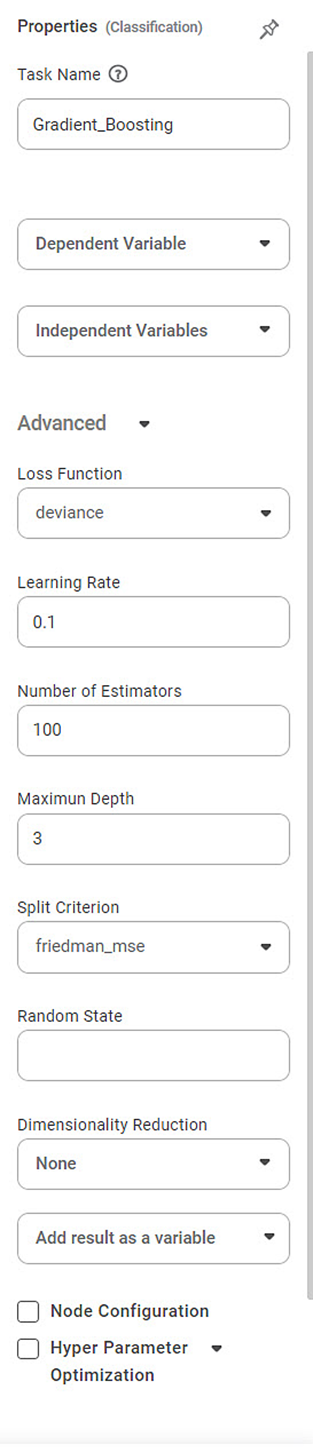
Properties of Gradient Boosting
Field | Description | Remark | |
| Run | It allows you to run the node. | - | |
| Explore | It allows you to explore the successfully executed node. | - | |
| Vertical Ellipses | The available options are
| - | |
Task Name | It is the name of the task selected on the workbook canvas. | You can click the text field to edit or modify the task name as required. | |
Dependent Variable | It allows you to select the dependent variable | You can choose only one variable, which should be Categorical type. | |
Independent Variable | It allows you to select the independent variable. |
| |
Advanced | Loss Function | It allows you to choose from 2 options: deviance & exponential | It is a function that maps an event or values of one or more variables onto an actual number. |
Learning Rate | It allows you to change the learning rate accordingly | It is a tuning parameter in an optimization algorithm that determines the step size at each iteration while moving towards a minimum of a loss function | |
Number of estimators | It allows you to select the number of estimators. | It is an equation for picking the best or most likely accurate data model based on observations. | |
Maximum Depth | It allows you to select the amount of the maximum depth. | It refers to the maximum number of levels or layers created in the boosting process. | |
Split Criterion | It allows you to select any of the options in the box. | It is a method to evaluate and select the best-split points when constructing decision trees within the boosting process. | |
Random State | It allows you to enter the value of the random state. | It refers to a parameter controlling the random number generation during training. | |
Example of Gradient Boosting
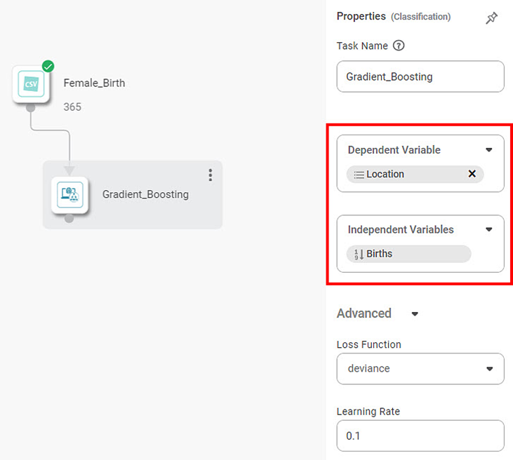
Here, we apply Gradient Boosting to the Female birth dataset in the example below. The independent variable is Births. The dependent variable is "Location."
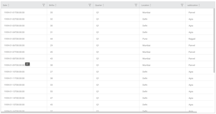
The figure given below displays the input data:
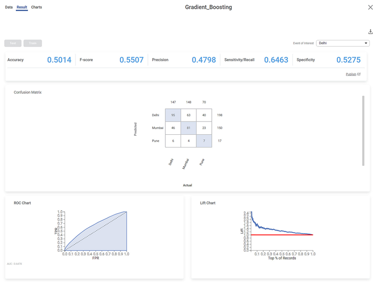
After using Gradient Boosting, the following results are displayed according to the Event of Interest
The result page displays the following sections.
- Key Performance Index
- Confusion Matrix
- Graphical Representation
Section 1 – Key Performance Index (KPI)
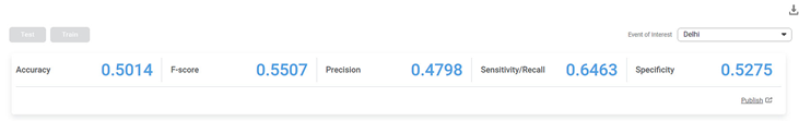
The Table given below describes the various parameters present on the Key Performance Index:
Field | Description | Remark |
Accuracy | Accuracy is the ratio of the total number of correct predictions made by the model to the full predictions. | The Accuracy is 0.5014. |
F-Score | F-score is a measure of the accuracy of a test. | It is also called the F-measure or F1 score. |
Precision | Precision is the ratio of the True positive to the sum of the True positive and False Positive. It represents positive predicted values by the model. | The precision for No is 0.4798 |
Sensitivity | It measures the test's ability to identify positive results correctly. | It is also called the True Positive Rate. |
Specificity | It gives the ratio of the correctly classified negative samples to the total negative pieces. | It is also called inverse recall. |
Section 2 – Confusion Matrix
The Confusion Matrix obtained is given below:
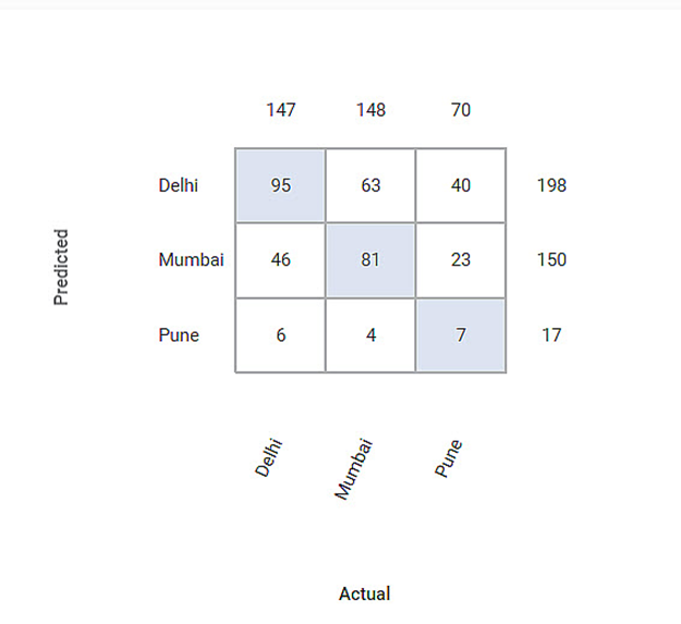
The Table given below describes the various values present in the Confusion Matrix:
Let us calculate the TP, TN, FP, and FN values for the class Delhi.
Field | Description | Remarks |
Predicted | It provides the predicted values from the classification model. | Here the predicted values for Delhi are 95. |
Actual | It gives the actual values from the result. | Here the actual values for Delhi are 95. |
True Positive | It gives the number of results that are genuinely predicted to be positive. The Actual Value and the predicted value should be the same. | Here TP value is 95. |
True Negative | It gives the number of results that are genuinely predicted to be negative. The sum of all the columns and rows except the values of that class that we are calculating the values for. | Here the TN value isTN = ( 81 + 23 + 4 + 7 )= (115) |
False Positive | It gives the number of results that are falsely predicted to be positive. The sum of the values of the corresponding columns except TP value. | Here FP value isFP = ( 63 + 40 )= ( 103 ) |
False Negative | It gives the number of results that are falsely predicted to be negative. The sum of values of the corresponding rows except for the TP value. | Here FN value is FN = ( 46 + 6 )= ( 52 ) |
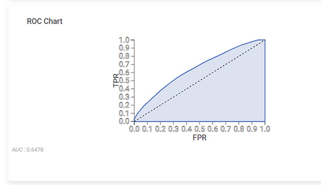
Section 3 – Geographical Representation
The Receiver Operating Characteristic (ROC) Chart for the Event of Interest is given below:
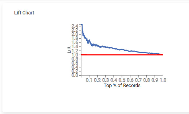
The Lift Chart obtained for the Event of Interest is given below:
The Table given below describes the ROC Chart and the Lift Curve:
Field | Description | Remark |
ROC Chart | The ROC curve is a probability curve that helps measure the performance of a classification model at various threshold settings. | The ROC curve is plotted with True Positive Rate on the Y-axis and False Positive Rate on the X-axis. |
Lift Chart | A lift is the measure of the effectiveness of a model. | A lift chart contains a lift curve and a baseline. |
Related Articles
Classification
Notes: The Reader (Dataset) should be connected to the algorithm. Missing values should not be present in any rows or columns of the reader. To find out missing values in a data, use Descriptive Statistics. Refer to Descriptive Statistics. If missing ...Extreme Gradient Boost Classification (XGBoost)
Extreme Gradient Boost is located under Machine Learning () in Classification, in the task pane on the left. Use the drag-and-drop method (or double-click on the node) to use the algorithm in the canvas. Click the algorithm to view and select ...Extreme Gradient Boost Regression (XGBoost)
XGBoost Regression is located under Machine Learning ( ) in Regression, in the left task pane. Use the drag-and-drop method to use the algorithm in the canvas. Click the algorithm to view and select different properties for analysis. Refer to ...AdaBoost in Classification
You can find AdaBoost under the Machine Learning section in the Classification category on Feature Studio. Alternatively, use the search bar to find the AdaBoost algorithm. Use the drag-and-drop method or double-click to use the algorithm in the ...Adaboost
Adaboost is located under Textual Analysis ( ) in Classification, in the left task pane. Use the drag-and-drop method to use the algorithm in the canvas. Click the algorithm to view and select different properties for analysis. Refer to Properties of ...