Holts-Winters Exponential Smoothing

Holts-Winters Exponential Smoothing

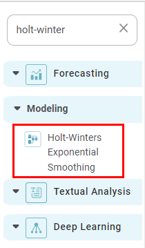
Holts-Winter Exponential Smoothing is located under Forecasting > Modeling > Holts-Winter Exponential Smoothing. Double-click or drag-and-drop the algorithm to use in the workbook canvas. Click the algorithm to view and select the different properties for analysis.
 

Properties of Holts-Winter Exponential Smoothing

The properties of Holts-Winter Exponential Smoothing are shown as figure below:


The table below describes the different fields present on the properties of Train-Test Split.

Field

Description

Remark


It helps to execute the node.

--


It helps to explore the successful node.

--


It displays the following options in the list view.

  • Run till node
  • Run from node
  • Publish as a model
  • Publish code

--

Task Name

It is the name of the task selected on the workbook canvas.

You can click the text field to edit or modify the task name as required.

Time ID Variable

It allows you to select the interval type variable for which we need to process the dependent or target variable's values.

  • Only one data field can be selected.
  • If selected, only an interval type variable should be selected.
  • Variables with numerical value are not available.

Target Variable

It allows you to select the experimental or predictor variable(s).

  • Only one data field can be selected.
  • Variables with only numerical values are available.

Group By

It allows you to select the variable for which you want to group the data.

  • Multiple data field can be selected.
  • Only categorical type variables are available.

Advanced


Trend

It represents the direction and rate of change in the underlying level of the time series data over time.

The available options are

  • None
  • add
  • mul
  • additive
  • multiplicative
    The default value is None.

Interval

It allows to select the interval for the accumulation of data in the accumulation test.

Available options are –

  • Day
  • Week
  • Month
  • Quarter
  • Year

    The default value is Month.

Damped Trend

A trend that gradually decreases over time, reflecting the expectation that the growth rate will slow down or plateau.

The available options are

  • True
  • False

Seasonal Period

  • It is a key parameter in time series analysis that represents the length of one complete cycle of seasonal variations in the data.
  • This period corresponds to the frequency at which the seasonal pattern repeats.

For example,

  • In monthly data, if there is an annual seasonal pattern, the seasonal period is 12 months.
  • In weekly data, if the pattern repeats every year, the seasonal period would be 52 weeks.

Seasonal

It specifies the type of seasonality to be used in the model.

The available options are

  • None
  • add
  • mul
  • additive
  • multiplicative
    The default value is None.

Initialization Method

It refers to the approach used to set the initial values for the level, trend, and seasonal components of the time series.

The available options are

  • None
  • estimated
  • heuristic
  • legacy-heuristic
  • known
    The default value is None.

Initial Level

It estimates the starting value of the time series, representing the baseline level from which trends and seasonal components are calculated.

--

Initial Trend

It is an estimate of the trend component at the start of the time series.

--

Initial Seasonal

estimates the values of the seasonal components for each period within the first full season of the time series.

--

Use Boxcox

It allows use of the box cox transformation to stabilize variance and make the data more normally distributed, which can improve the accuracy and reliability of the model.

The available options are

  • True
  • False
  • log
  • float
    The default value is False.

Missing

It provides the option to deal with the missing data.

The available options are

  • None
  • drop
    The default value is None.

Number of Periods of Forecasting

Enter the number of future time points for which predictions to be made using the model.

--

Bounds

It allows you to specify constraints for the optimization process when fitting the model.

The available options are:

  • DAMPING_TREND
  • SMOOTHING_SEASONAL
  • INITIAL_TREND
  • INITIAL_LEVEL

Example of Holt-Winters Exponential Smoothing

Consider a StockPrice dataset. It contains historical data of a stock's prices over a period. It contains a "Close" column on which we apply the transformation. A snippet of the input data is shown below.


We apply the Train Test Split to the input data and then apply the Holt Winter Exponential Smoothing to the Train Test Split node.

The figure below displays the properties pane with selected values.


Further, the result page displays,
  • Forecasting chart with predicted value.
  • Trained Model Parameters
  • Accuracy Parameters


    • Related Articles

    • Simple Exponential Smoothing

      To use Simple Exponential Smoothing, go to Forecasting > Modeling, and select Simple Exponential Smoothing. Use the drag-and-drop method or double-click to use the algorithm on the canvas. Click the algorithm to view and select different properties ...
    • Holt Exponential Smoothing

      Holt Exponential Smoothing is located under Forecasting > Modeling > Holt Exponential Smoothing. Double-click or drag-and-drop the algorithm to use in the workbook canvas. Click the algorithm to view and select the different properties for analysis. ...
    • Components in Forecasting

      Forecasting deals with the analysis and detection of trends in the time-series data. The components of forecasting are, Data Exploration: Data Exploration is used to explore the time-series data. It helps in identifying the underlying parameters ...
    • Parametric Distribution Fitting

      Parametric Distribution Fitting is located under Model Studio () in Statistical Analysis, in the left task pane. Use the drag-and-drop method to use the algorithm in the canvas. Click the algorithm to view and select different properties for ...
    • Inverse Cumulative Distribution Function

      Inverse Cumulative Distribution Function is located under Model Studio ( ) in Statistical Analysis, in the left task pane. Use the drag-and-drop method to use the algorithm in the canvas. Click the algorithm to view and select different properties ...