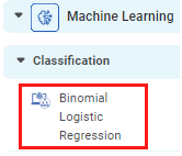
Binomial Logistic Regression is located under Machine Learning () in Data Classification, in the task pane on the left. Use drag-and-drop method to use the algorithm in the canvas. Click the algorithm to view and select different properties for analysis. Refer to Properties of Binomial Logistic Regression.

Properties of Binomial Logistic Regression

The available properties of Binomial Logistic Regression are as shown in the figure given below.

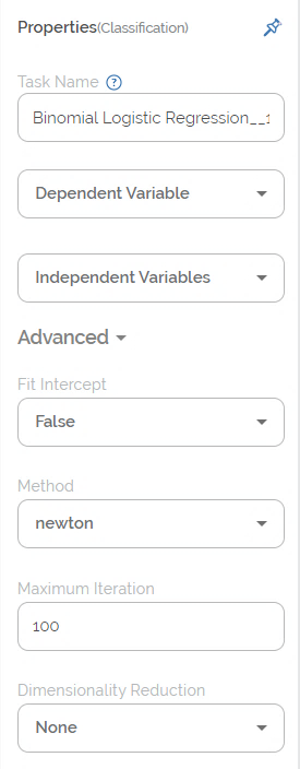
The table given below describes the different fields present in the properties of Binomial Logistic Regression.

Field	Description	Remark
Run	It allows you to run the node.	-
Explore	It allows you to explore the successfully executed node.	-
Vertical Ellipses	The available options are Run till node Run from node Publish as a model Publish code	-
Task Name	It displays the name of the selected task.	You can click the text field to edit or modify the name of the task as required.
Dependent Variable	It allows you to select the binary variable.	Any one of the available binary variables can be selected.
Independent Variable	It allows you to select the continuous variable.	Multiple variables can be selected. To select the type of data scaling for a variable, hover over the name of the variable and click the gear icon. You can select any one of the data scaling techniques.
Fit Intercept	It allows you select the fit intercept.	Fit Intercept is a Boolean parameter. It has two values, True and False. By default, the value is selected as True.
Method	It allows you to select the method (or solver).	It is the algorithm to be used in the optimization problem. The available methods are newton lbfgs powell cg ncg basinhopping minimize
Maximum Iteration	It allows you to select the maximum number of iterations to be performed on the data.	By default, the value is selected as 100. You can select any value for the number of iterations to be performed.
Dimensionality Reduction	It allows you to select the dimensionality reduction option. There are two parameters available None Principal Component Analysis (PCA)	If you select PCA, another field is created for inserting the variance value. Select a suitable value of variance.

The table given below describes the different fields present in the properties of Binomial Logistic Regression.

Field	Description	Remark
Task Name	It displays the name of the selected task.	You can click the text field to edit or modify the name of the task as required.
Dependent Variable	It allows you to select the binary variable.	Any one of the available binary variables can be selected.
Independent Variable	It allows you to select the continuous variable.	Multiple variables can be selected. To select the type of data scaling for a variable, hover over the name of the variable and click the gear icon. You can select any one of the data scaling techniques.
Fit Intercept	It allows you select the fit intercept.	Fit Intercept is a Boolean parameter. It has two values, True and False. By default, the value is selected as True.
Method	It allows you to select the method (or solver).	It is the algorithm to be used in the optimization problem. The available methods are newton lbfgs powell cg ncg basinhopping minimize
Maximum Iteration	It allows you to select the maximum number of iterations to be performed on the data.	By default, the value is selected as 100. You can select any value for the number of iterations to be performed.
Dimensionality Reduction	It allows you to select the dimensionality reduction option. There are two parameters available None Principal Component Analysis (PCA)	If you select PCA, another field is created for inserting the variance value. Select a suitable value of variance.

Interpretation from Binomial Logistic Regression

The interpretation of Binomial Logistic Regression properties is given below.

1. Dependent Variable:
   In Binomial Logistic Regression, the dependent variable must be a binary variable. For example, 1/0, True/False, Pass/Fail, Yes/No, and so on. Thus, the target (dependent) variable has only two possible outcomes.
   If there are no categorical (binary) variables in the given dataset, or you want to use a continuous variable as a binary variable, you can convert it into a binary variable. For this, follow the steps given below.
   
   1. On the home page, find the dataset, and click Edit.
   2. Hover over the numerical variable which you want to convert into categorical (binary) variable and click the gear icon (  ) corresponding to it.
   3. From the Variable Type drop down list, select Categorical.
   4. Click Done.
      In the updated dataset, the variable appears as a categorical variable.
   5. In the workbook/workflow, use drag and drop to reload the new dataset from the reader list.
      Now, if you explore the dataset, the converted variable appears in the data fields as a binary variable.
2. Independent Variable:
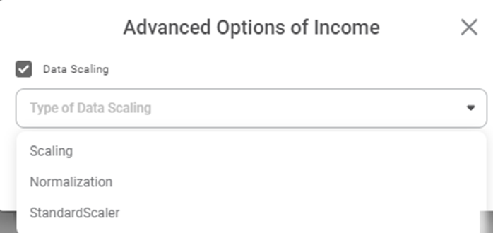
   Independent variables are continuous in nature. In Binomial Logistic Regression, we determine the probability or likelihood of the continuous independent variables falling in one of the two categories of the dependent (binary) variable.
   You can also use the data scaling option to standardize the range of data features. This may be required in case of data where the data values vary widely. The two types of data scaling possible are,
   
   • Scaling, in which the data is transformed such that the values are within a specific range [for example, (0,1)]
   • Normalization, in which data is transformed such that the values are described as a normal distribution, like a bell curve. In this case, the values are roughly equally distributed above and below the mean value.

   To select the scaling type, follow the steps given below.

   1. In the Properties column, hover over any independent variable and click the gear icon (  ).
   2. Select the Data Scaling check box.
   3. In the Type of Data Scaling drop down, select any one of the three types.
      

1. Fit Intercept: The fit intercept (also called constant or bias) decides whether the constant term in the linear equation will be added to the decision function. 
   If it is selected as True, the intercept is included in the model. If it is selected as False, the intercept is excluded from the model.

   Notes:

   Generally, fit intercept is included in models because it relaxes one of the Ordinary Least Squares (OLS) assumptions, that is, the zero mean of error term. However, owing to the possibility that the intercept may disturb some of the regularization techniques, it is usually either omitted or then manually added.

2. Method: Methods (also called solvers) are actually the algorithms which are used in the optimization problem. The solvers are selected depending upon different criteria and are used for different purposes. The list of available methods is given below.
   

   • Newton (for the Newton-Raphson method)
   • lbfgs (limited-memory BFGS with optional box constraints,. Where BFGS stands for Broyden-Fletcher-Goldfarb-Shanno)
   • powell (for the modified Powell's method)
   • cg (for conjugate gradient)
   • ncg (for Newton-conjugate gradient)
   • basinhopping (for global basin-hopping solver)
   • minimize (for generic wrapper of scipy minimize, which is BFGS by default)

3. Maximum Iteration: The maximum iteration decides the number of times you want to iterate the process.

4. Dimensionality Reduction: Dimensionality reduction removes redundant dimensions that generate similar or identical information, but do not contribute qualitatively to data accumulation. The options available in dimensionality reduction are given below.

• None, in which we do not perform dimensionality reduction.
• Principal Component Analysis (PCA), in which we perform dimensionality reduction and highlight the variability in the dataset.

Note:

When you select the PCA option, a Variance field appears. Insert a suitable value for variance

Example of Binomial Logistic Regression

In the example given below, the Binomial Logistic Regression is applied on a Credit Card Balance dataset. The independent variables are Income, Limit, Cards, Age, and Balance. The Gender is selected as the dependent (binary) variable.

The figure given below displays the input data.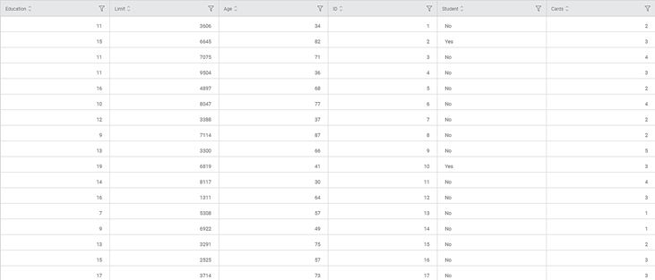

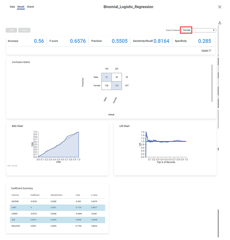
After using the Binomial Logistic Regression, the following results are displayed according to the Event of Interest, that is, either Male or Female.

Male: The Key Performance Index results obtained for the Event of Interest Male are given below.

The table given below describes the various parameters present on the Key Performance Index.

Field	Description	Remark
Sensitivity	It gives the ability of a test to correctly identify the positive results. Sensitivity = TP / (TP + FN) Where, TP = number of true positives FN = number of false negatives	It is also called as the True Positive Rate. The value of sensitivity for Male is 0.285.
Specificity	It gives the ratio of the correctly classified negative samples to the total number of negative samples. Specificity = TN / (TN + FP) Where, TN = number of true negatives FP = number of false positives .	It is also called inverse recall. The value of specificity for Male is 0.8164.
F-score	F-score is a measure of the accuracy of a test. It is the harmonic mean of the precision and the recall of the test. F-score = 2 (precision × recall) / (precision + recall) Where, precision = positive predictive value, which is the proportion of the positive values that are positive. recall = sensitivity of a test, which is the ability of the test to correctly identify positive results to get the true positive rate.	It is also called the F-measure or F1 score. The F-score for Male is 0.3846.
Accuracy	Accuracy is the ratio of the total number of correct predictions made by the model to the total predictions made. Accuracy = (TP + TN) / (TP + TN + FP + FN) Where, TP, TN, FP, and FN indicate True Positives, True Negatives, False Positives, and False Negatives respectively.	The Accuracy for Male is 0.56
Precision	Precision is the ratio of the True positive to the sum of True positive and False Positive. It represents positive predicted values by the model	The precision for male is 0.5914

The Confusion Matrix obtained for the Event of Interest Male is given below.

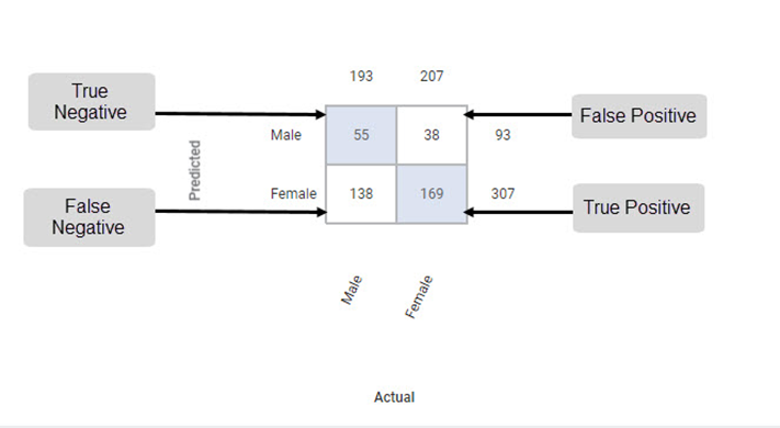
The Table given below describes the various values present in the Confusion Matrix.

Field	Description	Remark
Predicted	It gives the values that are predicted by the classification model.	The predicted values for Male and Female are Male – 93 Female - 307
Actual	It gives the actual values from the result.	The actual values for Male and Female are Male – 193 Female - 207
True Positive	It gives the number of results that are truly predicted to be positive.	The true positive count for Male is 169.
True Negative	It gives the number of results that are truly predicted to be negative.	The true negative count for Male is 55.
False Positive	It gives the number of results that are falsely predicted to be positive.	The false positive count for Male is 38.
False Negative	It gives the number of results that are falsely predicted to be negative.	The false negative count for Male is 138.

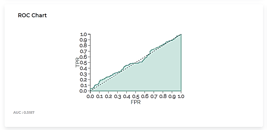
The Receiver Operating Characteristic (ROC) Chart for the Event of Interest Male is given below.

The Lift Chart obtained for the Event of Interest Male is given below.

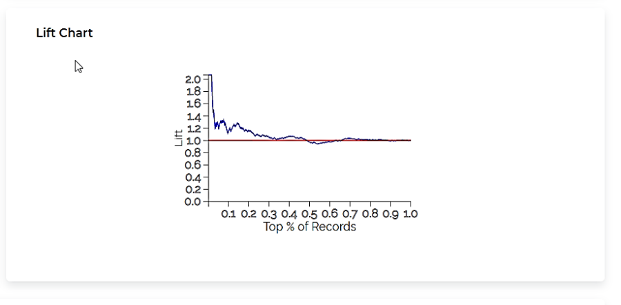
The table given below describes the ROC Chart and the Lift Curve

Field	Description	Remark
ROC Chart	ROC curve is a probability curve that helps in the measurement of the performance of a classification model at various threshold settings.	ROC curve is plotted with True Positive Rate on the Y-axis and False Positive Rate on the X-axis. We can use ROC curves to select possibly the most optimal models based on the class distribution. The dotted line is the random choice with probability equal to 50%, Area Under Curve (AUC) equal to 0.5, and the slope equal to 1. In the above graph, the ROC curve is very close to the dotted line.
Lift Curve	A lift is the measure of the effectiveness of a model. It is the ratio of the percentage gain to the percentage of random expectation at a given decile level. It is the ratio of the result obtained with a predictive model to that obtained without it.	A lift chart contains a lift curve and a baseline. It is expected that the curve should go as high as possible towards the top-left corner of the graph. Greater the area between the lift curve and the baseline, better is the model. In the above graph, the lift curve remains above the baseline up top 30% of the records and then becomes parallel to the baseline.

The Coefficient Summary obtained for the Event of Interest Male is given below.

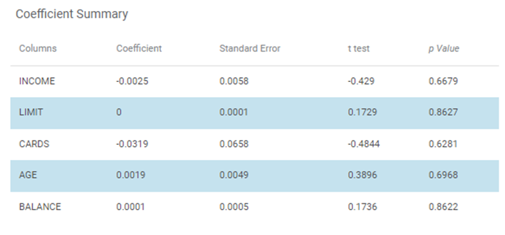
The table given below describes the various parameters present in the Coefficient Summary.

Field	Description	Remark
Columns	It displays the independent variables selected for Binomial Logistic Regression.	In the above example, Constant (CONST) Income, Limit, Cards, Age and Balance are the independent variables.
Coefficient	It is the degree of change in outcome variables for every unit change in the predictor variable.	_
Standard Error	It is used for testing whether the parameter is significantly different from 0.	_
t-test	It gives t-test statistic value used to test whether coefficients are significantly different from zero.	_
p-value	It helps to understand which coefficients has no effect in the regression model.	P-value < 0.05 is significant.

1. Female: The results obtained for the binary variable Female are given below.