Cumulative Distribution Function
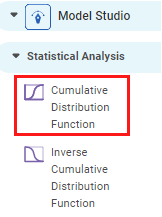
Cumulative Distribution Function is located under Model Studio (  ) in Statistical Analysis, in the left task pane. Use the drag-and-drop method to use the algorithm in the canvas. Click the algorithm to view and select different properties for analysis.
Refer to Properties of Cumulative Distribution Function.
Properties of Cumulative Distribution Function
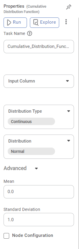
The available properties of the Cumulative Distribution Function are as shown in the figure below.
Field | Description | Remark | |
| Run | It allows you to run the node. | - | |
| Explore | It allows you to explore the successfully executed node. | - | |
| Vertical Ellipses | The available options are
| - | |
Task Name | It is the name of the task selected on the workbook canvas. | You can click the text field to edit or modify the name of the task as required. | |
Input Column | It allows you to select the variable to be selected as the input attribute. |
| |
Distribution Type | It allows you to select the type of distribution to be applied to the data. | There are two types of Distribution to select from:
| |
Distribution | It allows you to select the sub-type of the Distribution selected above. | The sub-types present in Continuous and Discrete Distribution are given in Description of Advanced Options for Distribution Type and Distribution Pairs. | |
Advanced | Node Configuration | It allows you to select the instance of the AWS server to provide control on the execution of a task in a workbook or workflow. | For more details, refer to Worker Node Configuration. |
In the Advanced options, algorithmic parameters for CDF also appear according to the pair of Distribution Type and Distribution selected. These parameters change according to the Distribution Type and Distribution selected.
For example, when you select the Cumulative Distribution Function node, the option for Distribution Type is Continuous and that for Distribution is Normal. In this case, the parameters that appear in the Advanced Options are Mean and Standard Deviation.
Advanced Options
The table below describes these two parameters.
Field | Description | Remark |
Mean | It allows you to select the mean value corresponding to the normal distribution. |
|
Standard Deviation | It allows you to select the value of standard distribution corresponding to the normal distribution. |
|
Distribution Type | Distribution | Parameter in Advanced Options | Description |
Continuous | Chi-squared | Degrees of Freedom |
|
Standard Exponential | — | The applicable parameters are already configured. | |
Exponential | Alpha (α) |
| |
F-distribution | Degree of Freedom 1 |
| |
Degree of Freedom 2 | |||
Gamma | Alpha (α) |
| |
Standard Normal | — | The applicable parameters are already configured. | |
Normal | Mean |
| |
Standard Deviation |
| ||
t | Degrees of Freedom |
| |
Standard Uniform | — | The applicable parameters are already configured. | |
Continuous Uniform | Lower Limit | The default value is 1. | |
Upper Limit |
| ||
Weibull_min | Shape Parameter |
| |
Weibull_max | Shape Parameter |
| |
Discrete | Bernoulli | Probability |
|
Binomial | Number of trials |
| |
Probability |
| ||
Geometric | Probability |
| |
Hypergeometric | Population Size |
| |
Number of successes |
| ||
Number of draws |
| ||
Poisson | lambda |
| |
Discrete Uniform | Lower Limit | The default value is 1. | |
Upper Limit | The default value is 2. |
Example of Cumulative Distribution Function
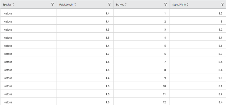
Consider the Iris dataset with columns of Sepal length, Sepal Width, Petal width and Species. A snippet of input data is shown in the figure below.
The selected values for properties and Advanced options for the Cumulative Distribution Function are given in the table below.
| Property | Value |
|---|---|
Input Column | Petal Width |
Distribution type | Discrete |
Distribution | Binomial |
Number of Trials | 10 |
Probability | 0.5 |
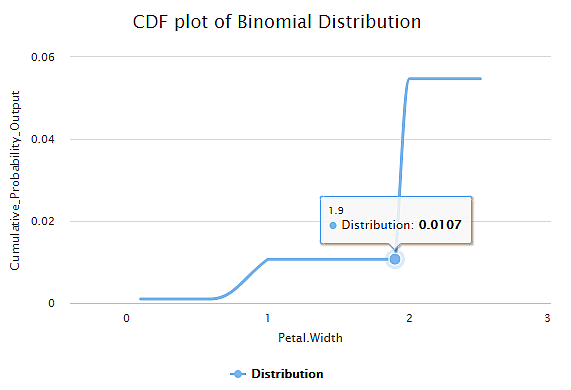
The Result page of the Cumulative Distribution Function is displayed in the figure below. The graph shows the variation in Cumulative Probability Output values for the given variable values (Petal Width) in the dataset.
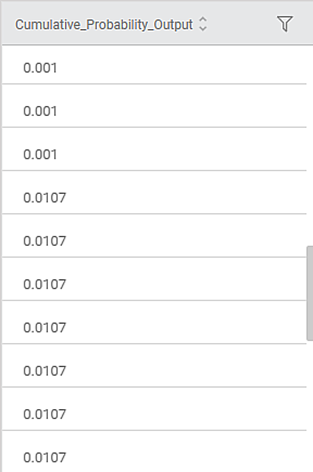
For example, the Petal Width value of 1.9 has a Cumulative Probability Output value of 0.0107.
The Data page of the Cumulative Distribution Function is displayed in the figure below. It shows a snippet of the Cumulative Probability Output values corresponding to Input Column values in tabular form. By default, the values of Petal Width are sorted and arranged in an ascending order.
Related Articles
Inverse Cumulative Distribution Function
Inverse Cumulative Distribution Function is located under Model Studio ( ) in Statistical Analysis, in the left task pane. Use the drag-and-drop method to use the algorithm in the canvas. Click the algorithm to view and select different properties ...Parametric Distribution Fitting
Parametric Distribution Fitting is located under Model Studio ( ) in Statistical Analysis, in the left task pane. Use the drag-and-drop method to use the algorithm in the canvas. Click the algorithm to view and select different properties for ...Dynamic Calculations
Dynamic Calculations is a part of the Expression function. Using Dynamic Calculations, you can define formulas to create new features from the existing features of the dataset. Dynamic Calculations is one of the features available in the Expression ...Custom Functions in RubiPython
Reading Data from File A sample Python code to read data from file is shown in the image below. The table below explains the above code snippet. Line of Code Result getReaderData(“datasetName”,“subdatasetName”) This custom function checks the type of ...Custom Functions in RubiPython
Reading Data from File A sample Python code to read data from file is shown in the image below. The table below explains the above code snippet. Line of Code Result getReaderData(“datasetName”,“subdatasetName”) This custom function checks the type of ...