Data Pivot
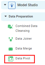
Data Pivot is located under Model Studio ( .png) ) in Data Preparation, in the left task pane. Use the drag-and-drop method to use the algorithm on the canvas. Click the algorithm to view and select different properties for analysis.
) in Data Preparation, in the left task pane. Use the drag-and-drop method to use the algorithm on the canvas. Click the algorithm to view and select different properties for analysis.
Refer to Properties of Data Pivot.
Properties of Data Pivot
The available properties of Data Pivot are shown in the figure below.
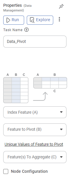
The depictions of tables and the change from one table structure to another are shown in the figure above. The elements A, B, and C of the first table are rearranged as shown in the second table.
The table below describes different fields present on the properties of Data Pivot.
Field | Description | Remark | |
|---|---|---|---|
Run | It allows you to run the node. | - | |
| Explore | It allows you to explore the successfully executed node. | - | |
| Vertical Ellipses | The available options are
| - | |
Task Name | It is the name of the task selected on the workbook canvas. |
| |
Index Feature (A) | It allows you to select the variable to be selected for the first column of the resultant table. |
| |
Feature to Pivot (B) | It allows you to select the variable(s) to be selected for the remaining columns of the resultant table. |
| |
Unique values of features to Pivot | It allows you to select unique variable values as column names in the resultant table. |
| |
Feature to Aggregate (C) | It allows you to select the variable to be aggregated based on the variable selected as Feature to Pivot (B). |
| |
Advanced | Node Configuration | It allows you to select the instance of the Amazon Web Services (AWS) server to provide control on the execution of a task in a workbook or workflow. | For more details, refer to Worker Node Configuration. |
Example of Data Pivot
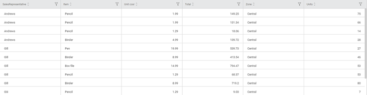
Consider a NewSalesData dataset containing information on the zone-wise sale of items by various sales representatives along with the unit cost and total. A snippet of the input data is shown in the figure below.
We select the following properties and apply Data Pivot.
Index Feature (A) | Item |
Feature to Pivot (B) | Zone |
Output Columns (unique values) | Central, East, and West |
Feature to Aggregate (C) | Total (Average) |
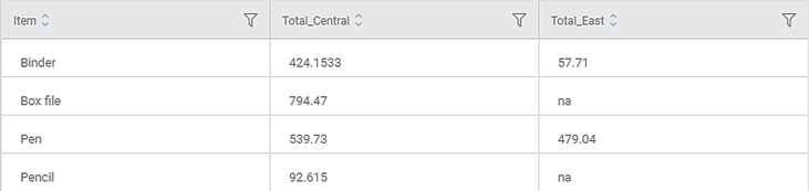
The figure below shows the resultant Pivoted table on the Data tab.
You can see that
- The table structure has changed from simple to cross, that is from a tall table to a wide one.
- The Total values are aggregated in second, third, and fourth columns by mean, for Central and East zones, respectively.
Related Articles
Data Pivot
Data Pivot is located under Model Studio in Data Preparation, in the left task pane. Use the drag-and-drop method to use the algorithm on the canvas. Click the algorithm to view and select different properties for analysis. Refer to Properties of ...Data Compare
Data Compare is located under Model Studio ( ) in Data Preparation, in the task pane on the left. Use the drag-and-drop method to use the algorithm in the canvas. Click the algorithm to view and select different properties for analysis. In the Data ...Live Data
Data visualization is the representation of data in the form of pictures, images, graphs, or any other form of visual illustration. In RubiThings, Live Data is visualized in the form of Line Chart, SolidGauge, and Speedometer. To fetch the live data, ...Data Merge
Data Merge is located under Model Studio ( ) in Data Preparation, in the task pane on the left. Use drag-and-drop method to use the algorithm in the canvas. Click the algorithm to view and select different properties for analysis. Properties of Data ...Data Merge
Data Merge is located under Model Studio ( ) in Data Preparation, in the task pane on the left. Use drag-and-drop method to use the algorithm in the canvas. Click the algorithm to view and select different properties for analysis. Properties of Data ...