Dynamic Calculations
Dynamic Calculations is a part of the Expression function. Using Dynamic Calculations, you can define formulas to create new features from the existing features of the dataset.
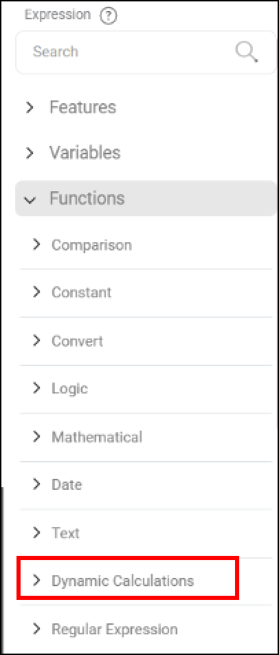
Dynamic Calculations is one of the features available in the Expression Builder on the Feature Definition page.
Types of Dynamic Calculation
The different types of Dynamic Calculations are explained in the table below.
Name and Calculation Type | Code Editor | Description |
Cumulative cumulative(, function="Sum", decimals=4) |
| It returns the cumulative value of the selected Feature based on the selected Function. Available values are:
|
Rolling Window rollingWindow(, function="Sum", direction="Backward", windowSize=1, decimals=4) |
| It returns the rolling value of the selected Feature based on the defined Window Size. Example: rollingWindow([Row ID], function="Mean", direction="Forward", windowSize=1, decimals=4) |
Difference diffData(, relativeTo="Previous", windowSize=1, decimals=4) |
| It returns the difference between two rows of the selected Feature based on the defined Window Size. Available Values are:
|
Percent Difference percentDiff(, relativeTo="Previous", windowSize=1, decimals=4) |
| It returns the percentage difference between two rows of the selected Feature based on the defined Window Size. Available Values are:
|
Percent From percentFrom(, relativeTo="Previous", windowSize=1, decimals=4) | Coming soon | Coming soon |
Rank rankData(, , method="Dense", order="ASC") |
| It returns the numerical data ranks of a Feature in the selected Order based on the selected Rank Method. Methods:
Order:
|
Lag lagData(, windowSize=1) |
| It returns the value from a previous row of the selected Feature based on the defined Window Size. |
Lead leadData(, windowSize=1) |
| It returns the value from the next row of the selected Feature based on the defined Window Size. |
The sections below explain each of these calculations in detail.
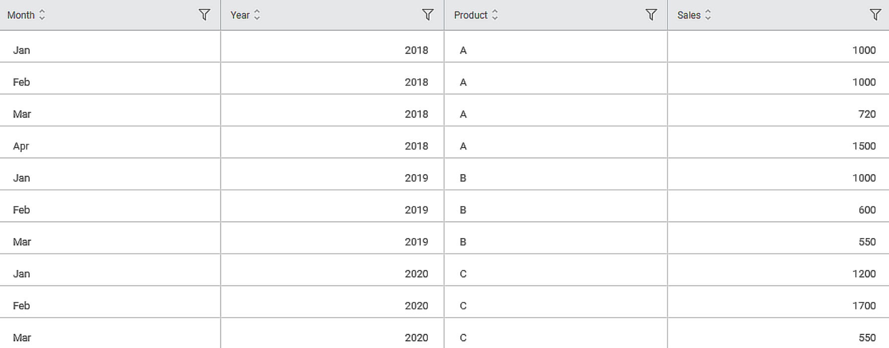
Consider the data snippet displayed in the below figure.
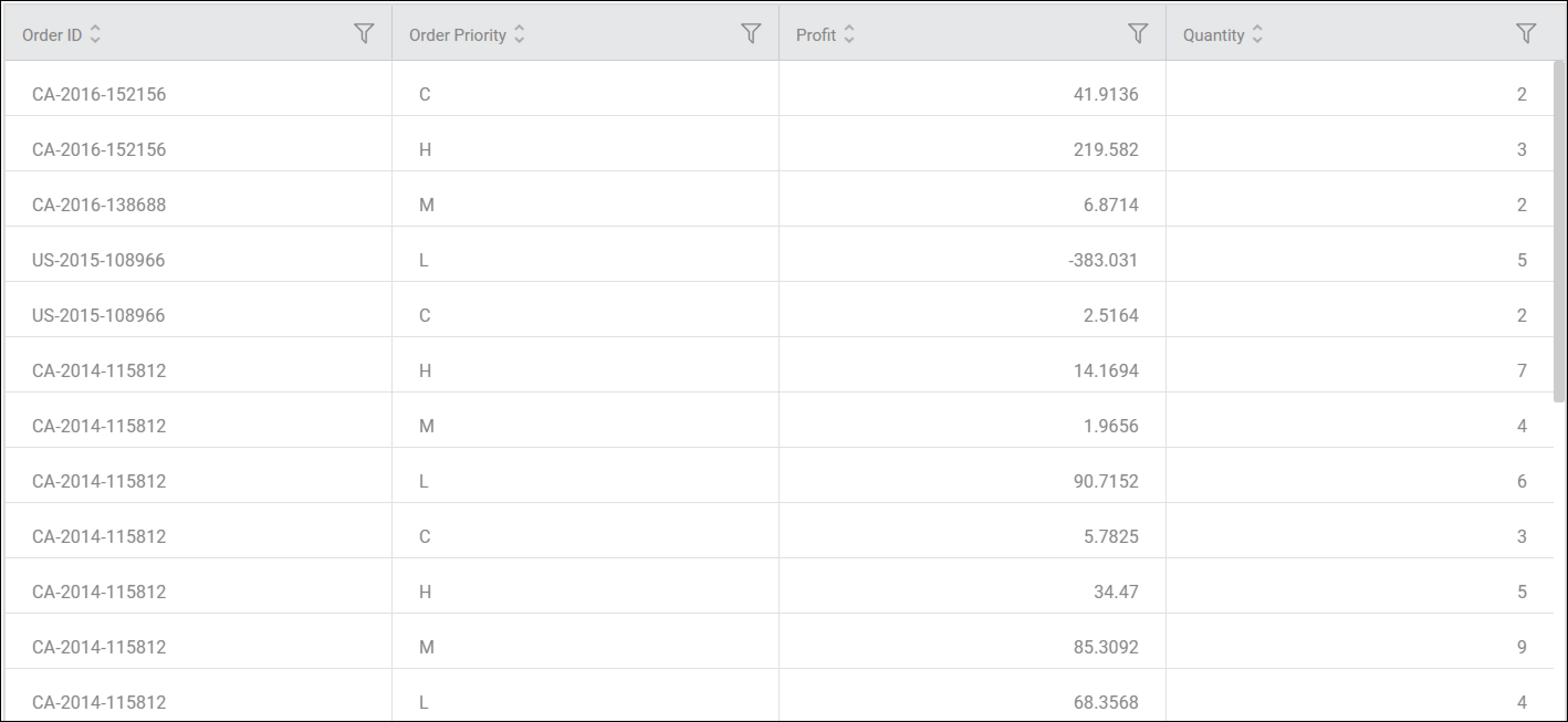
This input data is used in the examples of different types of Dynamic Calculations in the below sections.
Cumulative
The Cumulative expression provides the functionality to obtain a running value of a feature based on the selected function.
It can be used only on numerical features.
The elements in Cumulative expression are displayed in the figure below.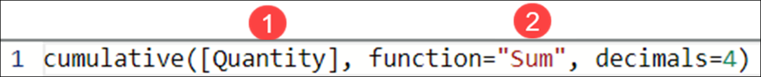
The table given below describes the elements in the Cumulative expression.
Sr. No. | Field Name | Description |
1 | Feature | This drop-down allows you to select a numerical feature from the selected dataset. |
2 | Function | It allows you to select the function to be performed on the selected feature. The available options are:
|
Consider the input dataset in Figure: Input Data Snippet. The table below describes the input fields selected on the Feature Definition page for Cumulative Expression.
Field | Value |
Input/Selected Feature | Quantity |
New Feature Name | Cumulative |
Variable Type of New Feature | Numerical |
Data Type of New Feature | Integer |
The output Data page of the Cumulative node displays an additional feature Cumulative, along with the existing features, as shown in the figure below.
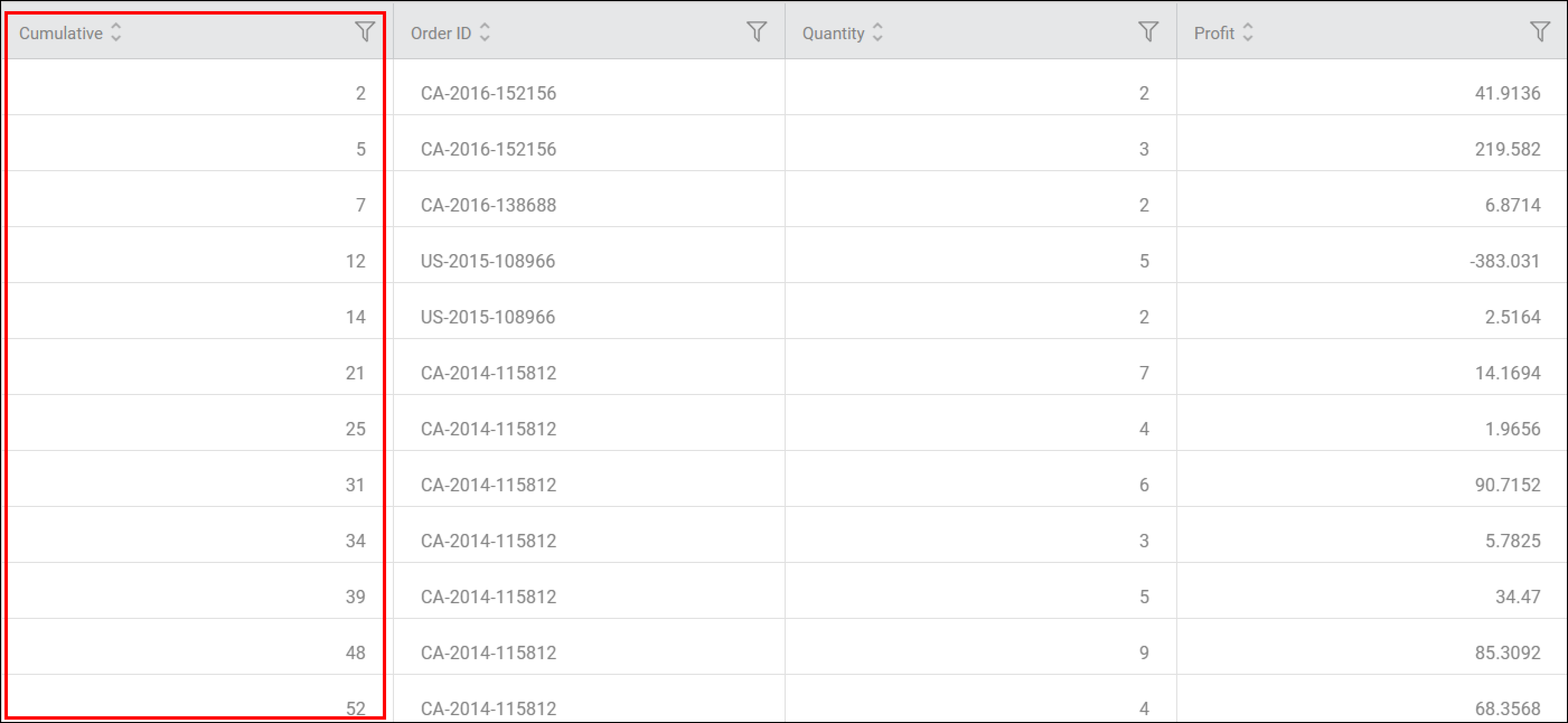
The new feature displays the result of the Cumulative calculations. Here, each cell in the new feature displays the sum of the previous cumulative value and the current row value.
The Cumulative value of the nth row is calculated as per the formula given below.
Cumulative Value = Selected_function(Current Row Value, Previous Cumulative Value)
- If the selected function is Sum, then Output = Sum(Current Row Value, Previous Cumulative Value).
- If the selected function is Mean, then Output = Mean(Current Row Value, Previous Cumulative Value).
- If the selected function is Min, then Output = Min(Current Row Value, Previous Cumulative Value).
- If the selected function is Max, then Output = Max(Current Row Value, Previous Cumulative Value).
In this example, the selected function is Sum, so the cumulative values are calculated as below –
First row - Same as the value of the original feature, 2.
Second row - [2] + [3] = [5]
Third row is - [5] + [2] = [7], and so on.
Rolling Window
Rolling Window is used to return the rolling value of the feature based on the defined window size.
You can use Rolling Window only on features with numerical values, and the output type of rolling window is also a numerical value. The two directions available in the Rolling Window expression are Forward and Backward.
The elements in the Rolling Window expression are displayed in the figure below.
The table given below describes the elements in the Rolling Window expression.
Sr No. | Field Name | Description |
1 | Feature | It allows you to select a numerical feature available in the selected dataset. |
2 | Function | It allows you to select the function to be performed on the selected feature. The available options are:
|
3 | Direction | It allows you to select the direction to consider while performing the rolling window calculation of the selected feature. The available directions are:
|
4 | Window Size | It allows you to enter an integer value as the window size. The minimum value for Window Size is 1, and the maximum value is (n – 1), where n is the total number of data points. |
Consider the input dataset in Figure: Input Data Snippet. The table below describes the input fields selected on the Feature Definition page for Rolling Window Expression.
Field | Value |
Input/Selected Feature | profit |
Function | Sum |
Direction | Forward |
Window size | 1 |
New Feature Name | Rolling_window |
Variable Type of New Feature | Numerical |
Data Type of New Feature | Float |
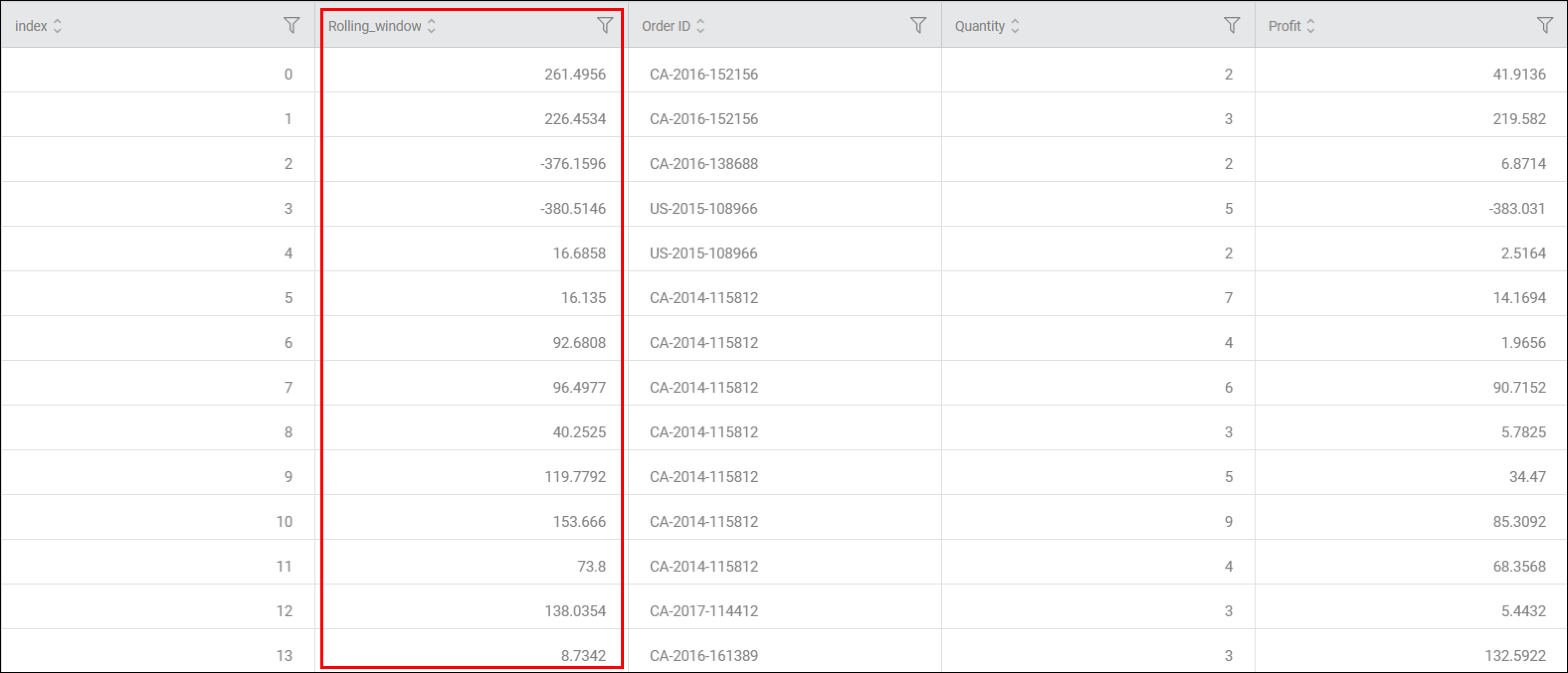
The output Data page of the Rolling Window node displays an additional feature (in this example, Rolling_window) along with the existing features, as shown in the figure below.
The Rolling Window value of the nth row is calculated as per the formula given below.
Rolling Window (n) = Selected_function(R1, R2)
Where,
R1 = Selected Feature Value (n)
R2 = Selected Feature Value[n + Window Size]; if the direction is Forward Or
R2 = Selected Feature Value[n - Window Size]; if the direction is Backward
For example, if the selected function is Mean, the direction is Forward, and the Window Size is 1.
Output = Mean(Current Row Value, Next Row Value)
In this example, the Selected Function is Sum, Direction is Forward, and Window Size is 1. So, the Rolling Window values are calculated as below -
First row: [41.9136] + [219.582] = [261.4956].
Second row: [219.582] + [6.8714] = [226.4534]
Third row: [6.8714] + [-383.031] = [-376.1596], and so on.
Difference
Difference expression returns the difference between values in two rows that are separated by Window Size. The output is a numerical value.
The elements in the Difference expression are displayed in the figure below.

The table given below describes the different elements in the Difference Expression.
Sr No. | Field Name | Description |
1 | Feature | It allows you to select the features available in the selected dataset. |
2 | Relative to | It allows you to select the relative value to calculate the difference. The available options are –
|
3 | Window Size | It allows you to enter an integer value as the window size. The minimum value for Window Size is 1, and the maximum value is (n – 1), where n is the total number of data points. |
Consider the input dataset in Figure: Input Data Snippet. The table below describes the input fields selected on the Feature Definition page for Difference Expression.
Field | Value |
Input/Selected Feature | Profit |
Relative To | Previous |
Window Size | 1 |
New Feature Name | Difference |
Variable Type of New Feature | Numerical |
Data Type of New Feature | Float |
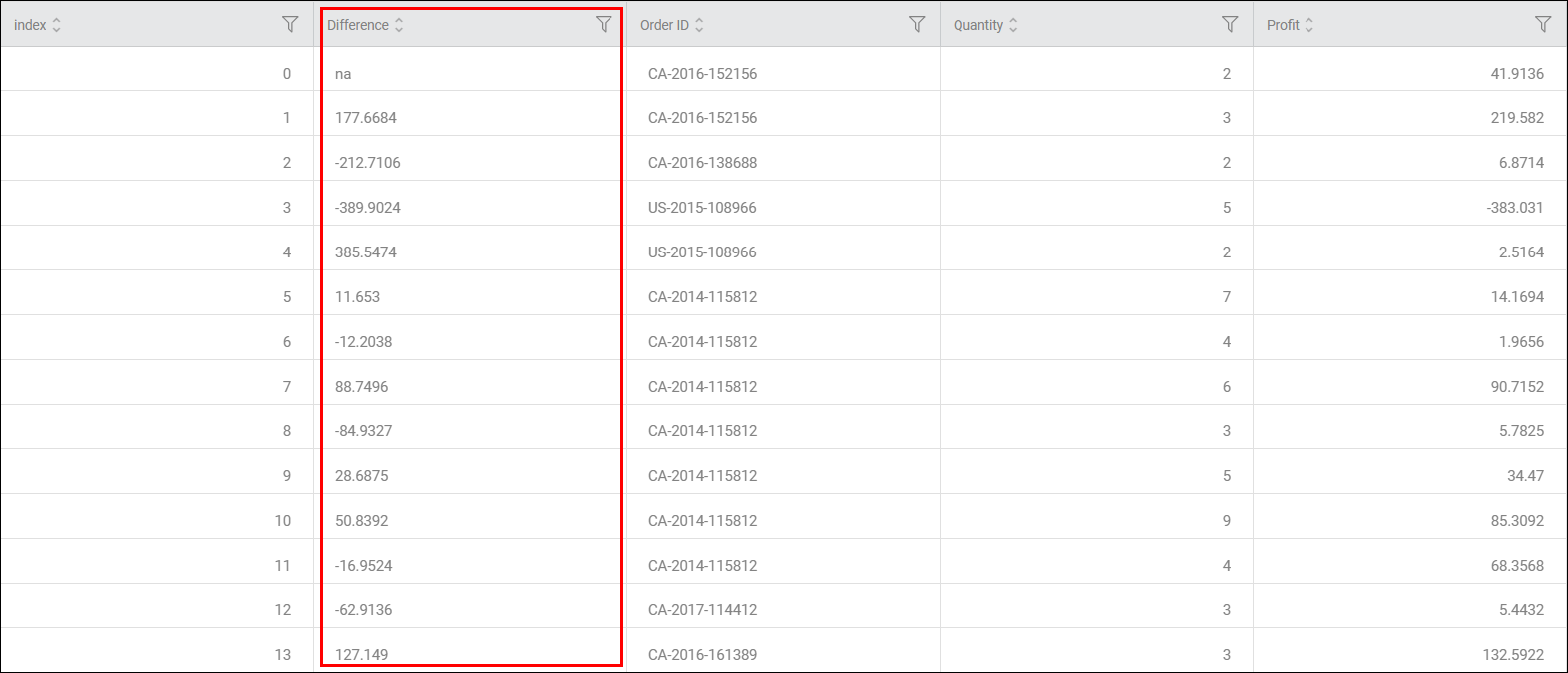
The output Data page of the Difference node displays an additional feature Difference along with the existing features, as shown in the figure below.
The Difference value of the nth row is calculated as per the formula given below.
Difference (n) = R1 - R2
Where,
R1 = Selected Feature Value (n)
R2 = Selected Feature Value[n - Window Size]; if the Relative To is Previous Or
R2 = Selected Feature Value[n + Window Size]; if the direction is Next Or
R2 = Selected Feature Value[First Row]; if the direction is First Or
R2 = Selected Feature Value[Last Row]; if the direction is Last Or
In this example, Relative To is Previous, and Window Size is 1. So, the Difference values are as below -
First row: na.
Second row: [219.582] - [41.9136] = [177.6684]
Third row: [6.8714] - [219.582] = [-212.7106], and so on.
Percent Difference
The Percent Difference expression returns the percentage change between values in two rows apart from each other by Window Size. The output is a numerical value.
The elements in the Percent Difference expression are displayed in the figure below.

The table given below describes the different elements in the Percent Difference Expression.
Sr No. | Field Name | Description |
1 | Features | It allows you to select the feature available in the selected dataset. |
2 | Relative to | It allows you to select the relative value for calculating the Percent Difference. The available options are –
|
3 | Window Size | It allows you to enter an integer value as the window size. The minimum value for Window Size is 1, and the maximum value is (n – 1), where n is the total number of data points. |
Consider the input dataset in Figure: Input Data Snippet. The table below describes the input fields selected on the Feature Definition page for Percent Difference Expression.
Field | Value |
Input/Selected Feature | Quantity |
New Feature Name | Percent_difference |
Variable Type of New Feature | Numerical |
Data Type of New Feature | Float |
Relative To | Previous |
Window Size | 1 |
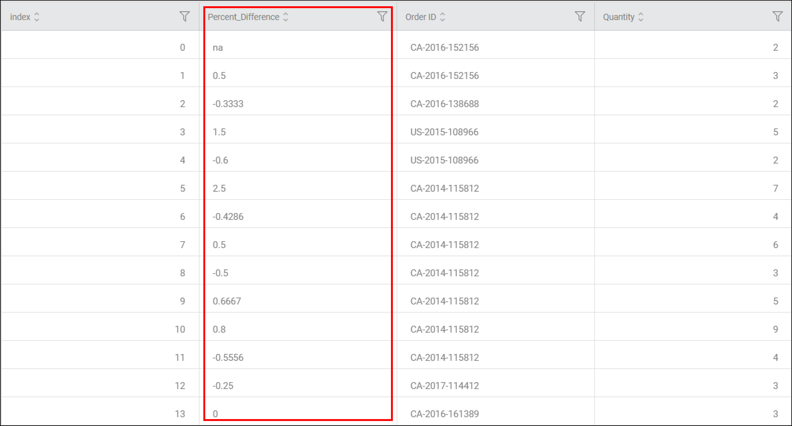
The output Data page of the Percent Difference node displays an additional feature Percent_difference along with the existing features, as shown in the figure below.
The Percent Difference value of the nth row is calculated as per the formula given below.
Percent Difference (n) = ((R1 – R2) / R2)
Where,
R1 = Selected Feature Value (n)
R2 = Selected Feature Value[n - Window Size]; if the Relative To is Previous Or
R2 = Selected Feature Value[n + Window Size]; if the direction is Next Or
R2 = Selected Feature Value[First Row]; if the direction is First Or
R2 = Selected Feature Value[Last Row]; if the direction is Last.
In this example, Relative To is Previous, and Window Size is 1. So, the Percent Difference values are as below -
First row: na.
Second row: (3-2) / 2 = 0.5
Third row: (2-3) / 3 = -0.3333, and so on.
Percent From
Percent From expression returns the percentage difference between values of two rows apart from the window size.
The elements in the Percent From expression are displayed in the figure below.

The table given below describes the different elements in the Percent From Expression.
Sr. No. | Field Name | Description |
1 | Features | It allows you to select the feature available in the selected dataset. |
2 | Relative to | It allows you to select the relative row for calculating the Percentage From. The available options are –
|
3 | Window Size | It allows you to enter an integer value as the window size. The minimum value for Window Size is 1, and the maximum value is (n – 1), where n is the total number of data points. |
Consider the input dataset in Figure: Input Data Snippet. The table below describes the input fields selected on the Feature Definition page for Percent From Expression.
Field | Value |
Input/Selected Feature | Total Profit |
New Feature Name | PercentFrom |
Variable Type of New Feature | Numerical |
Data Type of New Feature | Float |
Relative To | Previous |
Window Size | 1 |
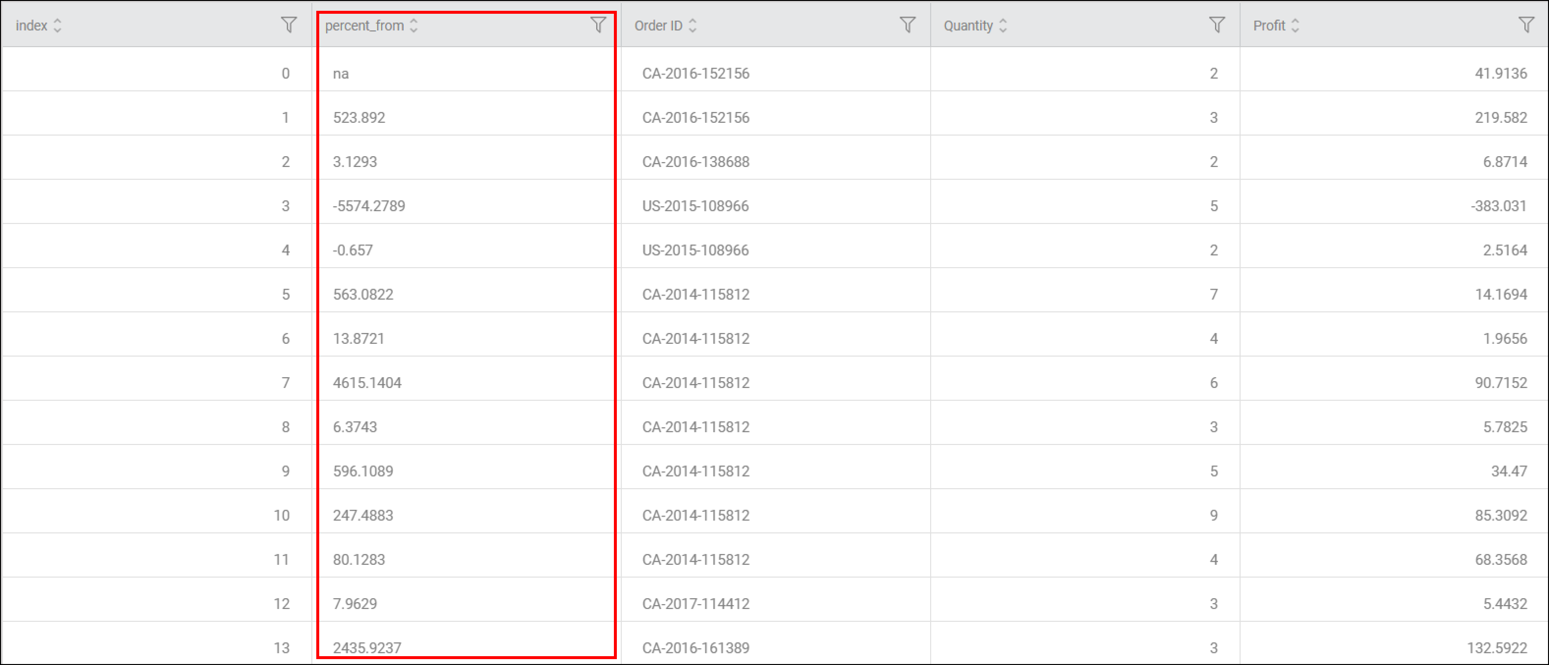
The output Data page of the Percent From node displays an additional feature, percentfrom, along with the existing features, as shown in the figure below.
The Percent From value of the nth row is calculated as per the formula given below.
Percent From (n) = ((R1 * 100)/R2))
Where,
R1 = Selected Feature Value (n)
R2 = Selected Feature Value[n - Window Size]; if the Relative To is Previous Or
R2 = Selected Feature Value[n + Window Size]; if the direction is Next Or
R2 = Selected Feature Value[First Row]; if the direction is First Or
R2 = Selected Feature Value[Last Row]; if the direction is Last Or
In this example, Relative To is Previous, and Window Size is 1. So, the, Percent From values are as below -
First row: na.
Second row: (219.582 * 100) / 41.9135 = 523.892
Third row: = (6.8714 * 100) / 219.582 = 3.1293, and so on.
Rank
The Rank expression returns the numerical rank of an input feature based on another feature. The output of Rank is an integer value.
The rank order is ascending or descending, and you can use this only on features with numerical values.
The elements in Rank expression are displayed in the figure below.
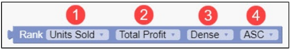
The table given below describes the different elements in Rank Expression.
Sr No. | Field Name | Description |
1 | Group By | It allows you to select a feature to perform the group by operation. |
2 | Feature | It allows you to select a feature available in the selected dataset. |
3 | Rank Method | It allows you to select the rank method to be used on the input feature. Available rank methods are:
|
4 | Rank Order | It allows you to select how your data should be sorted before allocating a rank value. The available options are –
|
Consider the input dataset shown in the figure below.
The output Data page of the Rank node displays an additional feature Year_Sales_Rank_Desc along with the existing features, as shown in the figure below.
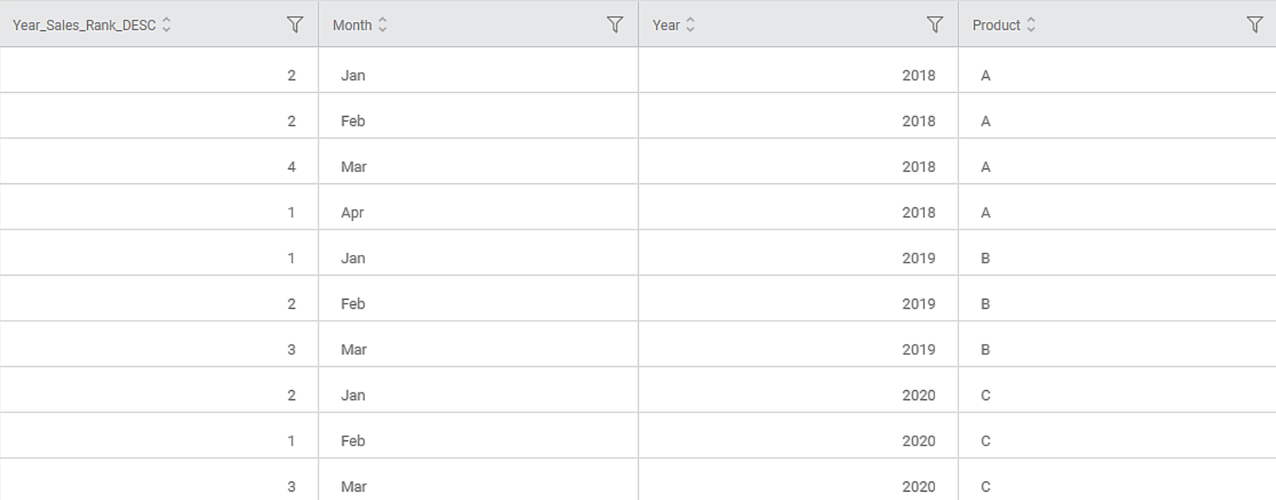
The newly created feature displays the rank of the Sales grouped by Year in descending order. In this example, since the method selected is Rank, Rubiscape assigns the rank number to each row in the partition. It skips the number for similar values. For example, in the above data, there are four values in the Year 2018 – 1000, 1000, 720, and 1500. The ranks of these values in descending order are 2, 2, 4, and 1.
The figure below shows the output of different rank methods. The names of the columns denote the rank method and sorting order.
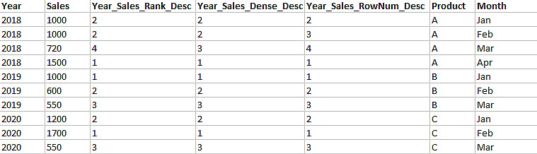
The newly added feature columns are explained below.
- Year_Sales_Rank_Desc displays ranks of Sales, grouped by Year using the Rank method, sorted by Descending
- Year_Sales_Dense_Desc displays ranks of Sales, grouped by Year using Dense method, sorted by Descending
- Year_Sales_RowNum_Desc displays ranks of Sales, grouped by Year using Row Number method, sorted by Descending
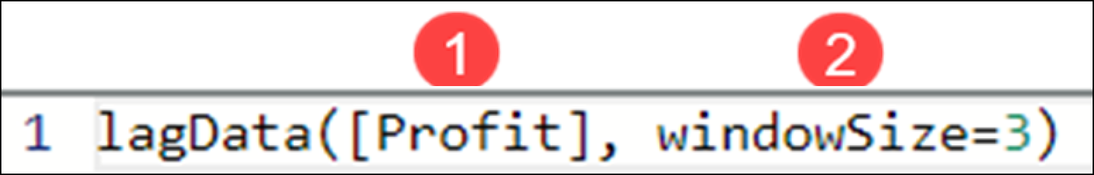
Lag
Lag expression is used to return the value from a row that is distanced from the current row by Window Size. Thus, you can enter any integer as window size. The elements in the Lag expression are displayed in the figure below.
The table given below describes the different elements in the Lag Expression.
Sr No. | Field Name | Description |
1 | Feature | It allows you to select the feature available in the selected dataset. |
2 | Window Size | It allows you to enter an integer value as the window size. The minimum value for Window Size is 1, and the maximum value is (n – 1), where n is the total number of data points. |
Consider the input dataset in Figure: Input Data Snippet. The table below describes the input fields selected on the Feature Definition page for Lag Expression.
Field | Value |
Input/Selected Feature | Total Profit |
New Feature Name | Lag |
Variable Type of New Feature | Numerical |
Data Type of New Feature | Float |
Window Size | 3 |
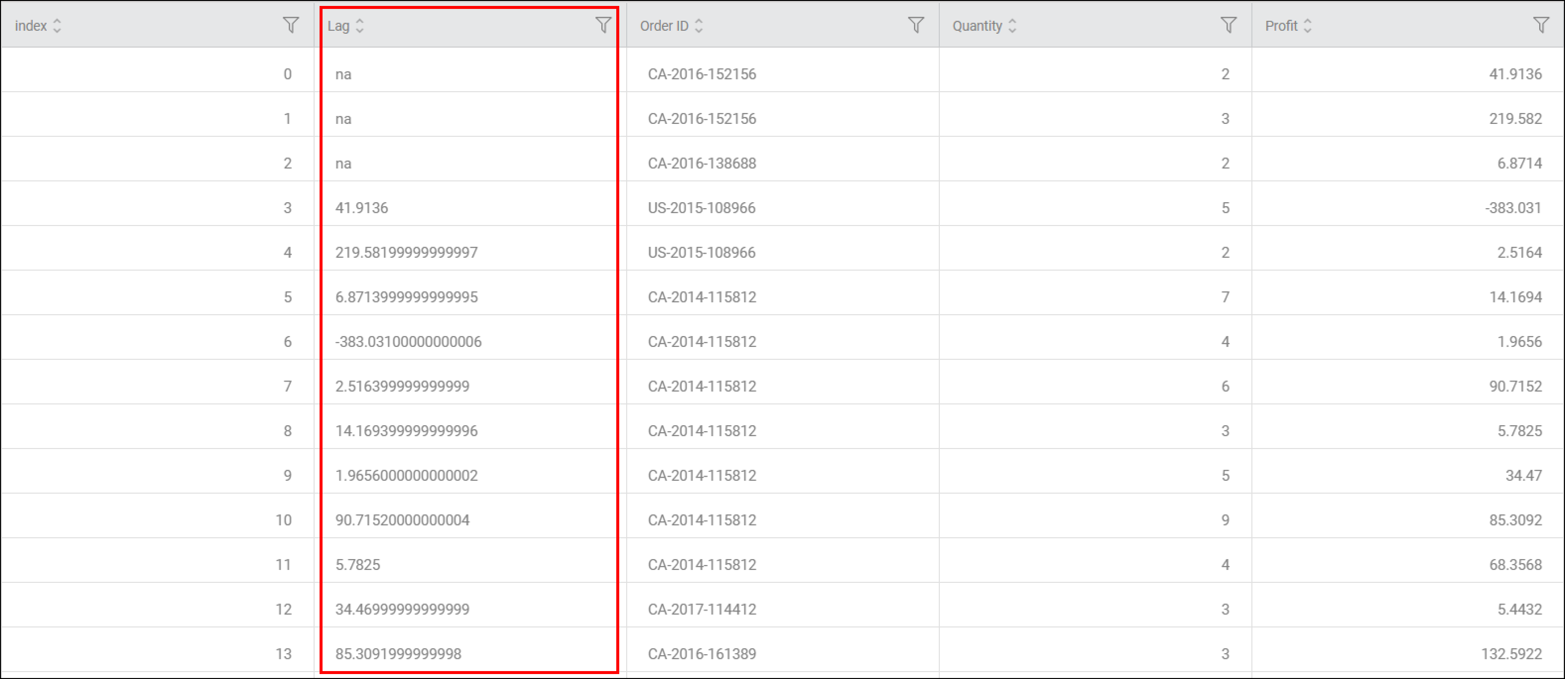
The output Data page of the Lag node displays an additional feature, Total Profit_Lag_3, along with the existing features, as shown in the figure below.
The Lag value of the nth row is calculated as per the formula given below.
Lag (n) = R[n - Window Size]
Where,
R = Selected Feature Value
In this example, the Window Size is 3. So, the, Lead values are as below -
First Row: Lag(1) = R[1 - 3] = na.
Second row: Lag(2) = R[2 - 3] = na
Third row: Lag(3) = R[3 - 3] = na
Fourth row: Lag(4) = R[4 - 3] = R1 = 41.9136
Fifth row: Lag(5) = R[5 - 3] = R2 = 219.582, and so on.
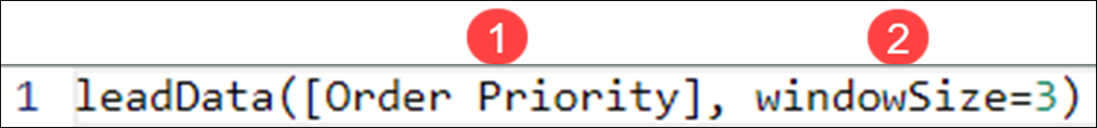
Lead
Lead expression is used to return the value from the next row, separated by Window Size. The elements in Lead expression are displayed in the figure below.
The table given below describes the different elements in the Lead Expression.
Sr No. | Field Name | Description |
1 | Feature | It allows you to select the feature available in the selected dataset. |
2 | Window Size | It allows you to enter an integer value as the window size. The minimum value for Window Size is 1, and the maximum value is (n – 1), where n is the total number of data points. |
Consider the input dataset in Figure: Input Data Snippet. The table below describes the input fields selected on the Feature Definition page for Lead Expression.
Field | Value |
Input/Selected Features | Priority |
Window Size | 3 |
New Feature Name | Lead |
Variable Type of New Feature | Categorical |
Data Type of New Feature | Numerical |
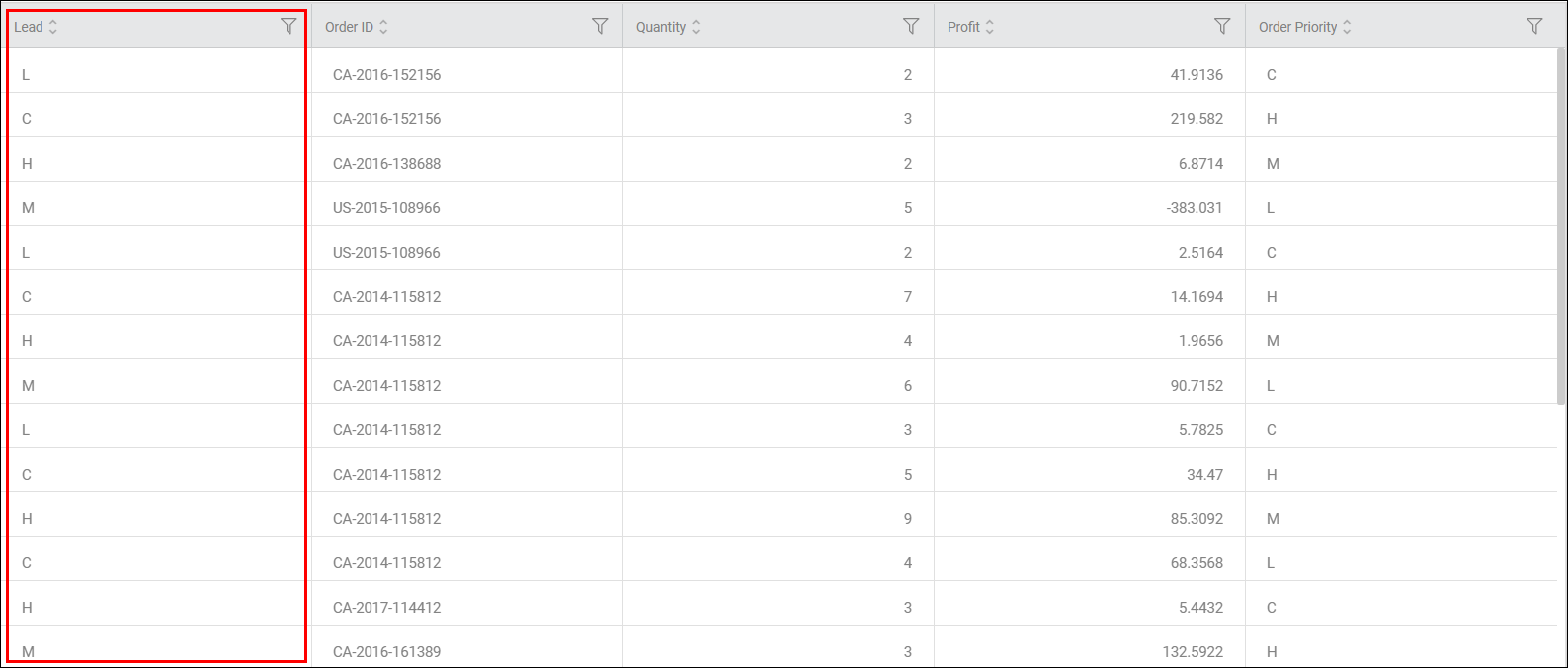
The output Data page of the Lead node displays an additional feature, Lead, along with the existing features, as shown in the figure below.
The Lead value of the nth row is calculated as per the formula given below.
Lead (n) = R[n + Window Size]
Where,
R = Selected Feature Value
In this example, the Window Size is 3. So, the, Lead values are as below -
First Row: Lead(1) = R[1+3] = R4 = L.
Second row: Lead(2) = R[2+3] = R5 = C
Third row: Lead(3) = R[3+3] = R6 = H
Notes: |
|

Related Articles
Percentage Calculations
For widgets like pie charts and donut charts, it is sometimes required to display the values as a percentage of the share of each section in the total share. For this, Rubiscape provides a Percentage functionality alongside the Aggregation methods to ...Expression
Expression is located under Model Studio ( ) in Data Preparation, in the Task Pane on the left. Use the drag-and-drop method to use the feature in the canvas. Click the feature to view and select different properties for analysis. Refer to Properties ...Expression
Expression is located under Model Studio ( ) in Data Preparation, in the Task Pane on the left. Use the drag-and-drop method to use the feature in the canvas. Click the feature to view and select different properties for analysis. Refer to Properties ...Calculated Columns in RubiSight
RubiSight provides a function to add a new column that is not originally present in your dataset. You can create a new column by doing some calculations on the existing columns. RubiSight uses the Expression function for creating a new column using ...Scrollbar Support in Charts
Scrollbar support allows users to handle large datasets and crowded visuals by enabling horizontal or vertical scrolling on charts. This ensures better readability and avoids overlapping of data points and labels. Overview Enables scrolling on X-axis ...