Factor Analysis
Factor Analysis is located under Model Studio ( 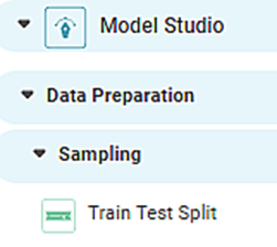 ) in Data Preparation, in the left task pane. Use the drag-and-drop method to use the algorithm in the canvas. Click the algorithm to view and select different properties for analysis.
Refer to Properties of Factor Analysis.
- Define the problem statement as to why you want to perform Factor Analysis
- Construct the Correlation Matrix
- Determine the Pearson Correlation between variables and identify which variables are correlated.
- Decide the method to be taken up for Factor Analysis
- Rotation for Varimax
- Maximum Likelihood
- Determine the number of relevant factors for the study. For example, you have a set of seven variables, and you want to reduce them to three. It is an individual decision based on the dataset and analytical requirements. (This is mostly determined using the trial and error methodology)
- Rotate the factors and interpret the results.
Properties of Factor Analysis
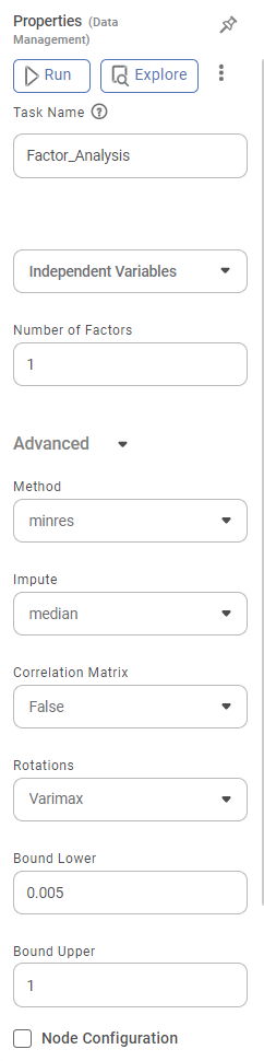
The available properties of the Factor Analysis are shown in the figure below.
The table below describes the different fields present on the Properties pane of the Chi-Square Goodness of Fit Test.
Field | Description | Remark | |
|---|---|---|---|
| Run | It allows you to run the node. | - | |
| Explore | It allows you to explore the successfully executed node. | - | |
| Vertical Ellipses | The available options are
| - | |
Task Name | It is the name of the task selected on the workbook canvas. |
| |
Independent Variable | It allows you to select the unknown variables to determine the factors. |
| |
Number of Factors | It allows you to select the number of factors you want to reduce the number of variables. |
| |
Advanced | Scores | It allows you to select the factor score for Factor Analysis. |
|
Rotations | It allows you to select the factor rotation method. |
| |
Node Configuration | It allows you to select the instance of the AWS server to provide control over the execution of a task in a workbook or workflow. | For more details, refer to Worker Node Configuration. | |
Results of Factor Analysis
The following table elaborates on the findings obtained from Factor Analysis.
Result | Significance | ||||||||
Loadings |
| ||||||||
KMO Test (Kaiser-Meyer-Olkin Test) |
Note: Practically, a KMO accuracy value above 0.5 is also considered acceptable for the validity of the test. Below 0.5, the value indicates that more data collection is essential since the sample is inadequate.| | ||||||||
Uniqueness |
| ||||||||
Communalities |
Practically, the values of communality extraction for a variable should be greater than 0.5. You can remove the variable and re-run the Factor Analysis in such a case. Note: However, values of 0.3 and above are also considered depending on the dataset. | ||||||||
Scree Plot |
| ||||||||
Bartlett Test of Sphericity |
|
Example of Factor Analysis
Consider a Hyundai Stock price dataset.
A snippet of the input data is shown in the figure given below.
For applying Factor Analysis, the following properties are selected.
Independent Variables | Open, High, Low, Close and so on |
Number of Factors | 4 |
Scores | None |
Rotation | Varimax |
The image below shows the Results page of the Factor Analysis.
We first look at the Bartlett Test of Sphericity results on the Results page, followed by the Scree Plot. The statistics and results obtained in this test is crucial to decide whether the Factor Analysis is required.
Bartlett's Test of Sphericity tells you whether you can go ahead with the Factor Analysis for data reduction. KMO test tells you whether the Factor Analysis is appropriate and accurate.
Bartlett Test of Sphericity:
- The Approximate value of Chi-Square = 48478.6146
- Degrees of Freedom (df) = 6
- Sigma (sig) = 0
Inference:
- Since the sigma value (0) is less than the p-Value (assumed as 0.05), the dataset is suitable for data reduction, in our case,Factor Analysis.
- It also indicates a substantial amount of correlation within the data.
KMO Test:
- You can see the individual KMO values for each variable.
- It is 7749for Open, 0.7745 for High, and so on.
- The overall KMO accuracy is 0.7798 (greater than 0.6).
Inference:
- Since the individual KMO scores for each variable are greater than 0.6, the individual data points are adequate for Sampling.
- Since the overall KMO score is greater than 0.6, the overall Sampling is adequate.
After the results from these two tests are analyzed, you can study other results. Among the remaining, you first analyze the communality extraction values for various variables.
Communalities:
- You can see the communality extraction score for each variable.
- It is 0.9974 for Open, 0.9982 for High, and so on.
- It is maximumfor High (0.9982) and minimum for Close (0.995).
Inference:
- The closer the communality is to one (1), the better is the variable explained by the factors.
- The closer the communality extraction values for variables, the better the chances of the variables belonging to a group (or community) and having a communal variance.
- For example, High, Low, and Close have high chances of belonging to a group.
Loadings:
- You can see the variance values of a variable as determined by each factor.
- For example, the variance of variable Open is better explained by factor F0 (0.998) compared to F2 (-0.0322).
- The factor loading scores indicate which variables fall into which factor category to be combined.
Notes: |
|
Uniqueness:
- You can see the uniqueness extraction values for each variable.
- It is 0.0026 for Open, 0.0018 for High, and so on.
- It is maximum for Open (0.0026) and minimum for Adj. Close (0.005).
- Uniqueness is calculated as '1- Communality'. It means that more communal is a variable, less is its uniqueness.
- Thus, Open is the most unique, while Close is the least unique value.
Correlation Plot:
- It gives the values of Pearson correlation for all the variables.
- A value of Pearson correlation closer to one (1) indicates a strong correlation between two variables, while a value close to zero (0) indicates a weak correlation.
Scree Plot:
- It plots the eigenvalues of factors against the factor number.
- It displays PC (Principal Component) value for components.
Related Articles
Factor Analysis
Factor Analysis is located under Model Studio ( ) in Data Preparation, in the left task pane. Use the drag-and-drop method to use the algorithm in the canvas. Click the algorithm to view and select different properties for analysis. Refer to ...Local Outlier Factor
Local Outlier Factor is located under Machine Learning ( ) in Anomaly Detection, in the task pane on the left. Use the drag-and-drop method (or double-click on the node) to use the algorithm in the canvas. Click the algorithm to view and select ...Basic Sentiment Analysis
Basic Sentiment Analysis is located under Textual Analysis ( ) in Sentiment, in the task pane on the left. Use drag-and-drop method to use algorithm in the canvas. Click the algorithm to view and select different properties for analysis. Refer to ...Basic Sentiment Analysis
Basic Sentiment Analysis is located under Textual Analysis ( ) in Sentiment, in the task pane on the left. Use drag-and-drop method to use algorithm in the canvas. Click the algorithm to view and select different properties for analysis. Refer to ...Process Capability Analysis
Process Capability Analysis is located under Model Studio ( ) under Statistical Analysis, in the left task pane. Use the drag-and-drop method to use the algorithm in the canvas. Click the algorithm to view and select different properties for ...