Local Outlier Factor
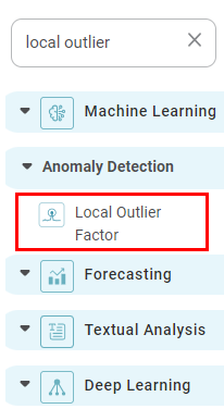
Local Outlier Factor is located under Machine Learning (  ) in Anomaly Detection, in the task pane on the left. Use the drag-and-drop method (or double-click on the node) to use the algorithm in the canvas. Click the algorithm to view and select different properties for analysis.
Refer to Properties of Local Outlier Factor.
Properties of Local Outlier Factor
The available properties of the Local Outlier Factor are as shown in the figure given below.
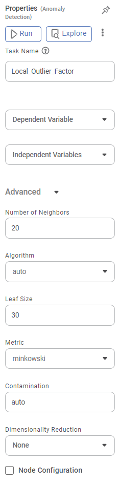
The table given below describes the different fields present on the Properties pane of the Local Outlier Factor.
Field | Description | Remark | |
| Run | It allows you to run the node. | - | |
| Explore | It allows you to explore the successfully executed node. | - | |
| Vertical Ellipses | The available options are
| - | |
Task Name | It displays the name of the selected task. | You can click the text field to edit or modify the name of the task as required. | |
Dependent Variable | It allows you to select the variable for which you need to perform the task. |
| |
Independent Variables | It allows you to select the experimental or predictor variable(s). | Multiple data fields can be selected. | |
Advanced | No. of Neighbors | It allows you to enter the number of neighboring data points. |
|
Algorithm
| It allows you to select the algorithm used for the search for the Nearest Neighbor. |
| |
Leaf Size
| It allows you to enter the number of leaf nodes. |
| |
Metric | It allows you to select the metric function used to define the distance between two points in a dataset. |
| |
Contamination | It determines the proportion of the points with the highest LOF scores (points that are most isolated) to be predicted as anomalies. |
| |
Dimensionality Reduction | It allows you to select the dimensionality reduction technique. Principal Component Analysis (PCA) maps the data linearly to a lower-dimensional space to maximize the variance of the data in the low-dimensional representation. |
| |
Variance | It allows you to enter the variance value. |
| |
Example of Local Outlier Factor
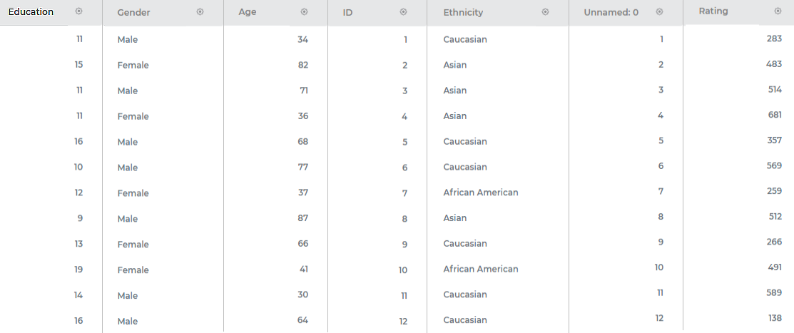
Consider a dataset Credit Card Balance with 13 features and 400 rows. A snippet of the input data is shown in the figure given below.
Property | Value |
Dependent Variable | Married |
Independent Variables | ID, Income, Limit, Rating, Cards, Age, Education, Balance |
No. of Neighbors | 20 |
Algorithm | auto |
Leaf Size | 30 |
Metric | Minkowski |
Contamination | auto |
Dimensionality Reduction | None |
The Result page of the Local Outlier Factor is shown in the figure given below.
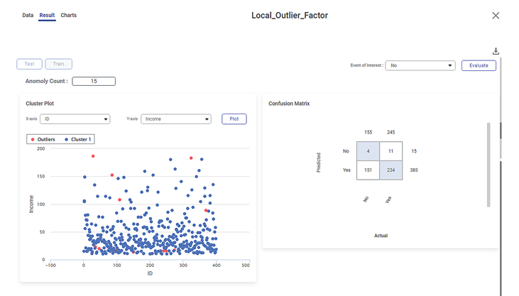
The Result page initially displays the Cluster Plot based on the default combination of features in the X-axis and Y-axis data fields. To plot a Cluster Plot for different combinations of features, select the respective features from the X-axis and Y-axis drop-downs.
| If you try to plot the Cluster Plot with the same features in the X-axis and Y-axis data fields, then Rubiscape gives an error. |

You can also view the Confusion Matrix based on the Event of Interest states of the selected dependent variable. Here, the dependent variable selected is Married, and its Event of Interest states are No and Yes.
To view the Confusion Matrix,
- Select either of the values from the Event of Interest drop-down.
- Click Evaluate, located in the top-right corner.
The Confusion Matrix is displayed on the right-hand side of the Result page.
The colored boxes in the Confusion Matrix represent the predicted values, while the white boxes represent the error values.
|
|
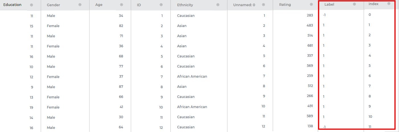
The output Data page displays two more columns, Label and Index, along with the existing 13 features in the LOF result. A snippet of the output data of 15 columns, displayed on the Data page, is shown in the figure below.
|
|
Interpretation of Result of Local Outlier Factor
The figure given below shows the Cluster Plot displayed on the LOF Result page.
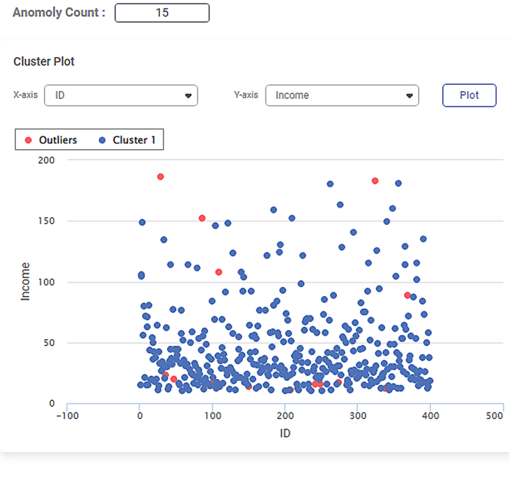
Some of the key observations from the Cluster Plot are listed below.
- The independent variable or label selected in the X-axis data field is
- The independent variable or label selected in the Y-axis data field is Income.
- The Cluster Plot is plotted between the two labels, one on X-axis (Age) and the other on Y-axis (Income).
- The blue dots in the plot represent the cluster of data points in the dataset of 400 data points.
- The red dots in the plot represent the local outliers in the cluster of data points.
The figure given below shows the Confusion Matrix displayed on the LOF Result page.
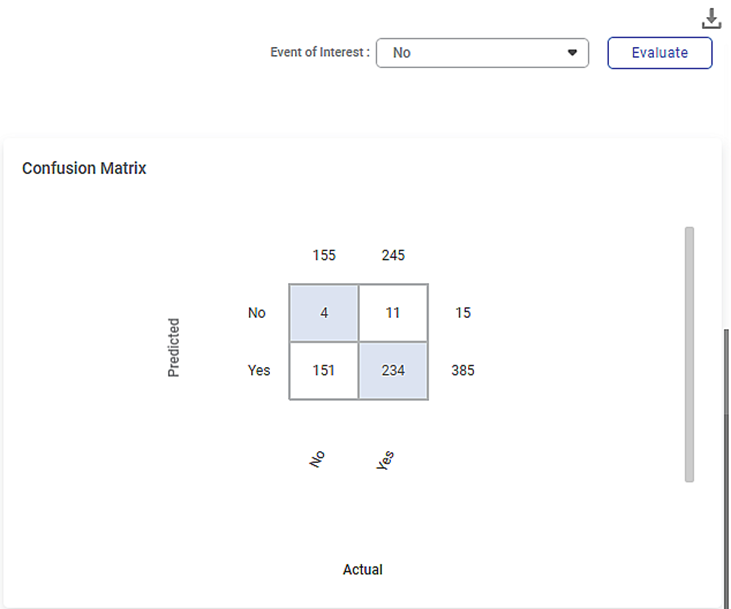
Some of the key observations from the Confusion Matrix evaluated for the selected dataset (of 400 data points) are listed below.
- The Confusion Matrix is evaluated for the value No selected from the Event of Interest drop-down.
- The blue boxes represent the predicted values.
The white boxes represent the error values.
The table below briefly explains what the values in each of the quadrants of the Confusion Matrix.
Quadrant
Quadrant Value
Description
First (blue)
4
The predicted values of No out of the actual No values (155).
Second (white)
11
The error values of Yes out of the actual Yes values (245).
Third (white)
151
The error values of No out of the actual No values (155).
Fourth (blue)
234
The predicted values of Yes out of the actual Yes values (245).
- The value 385 represents the number data points in a cluster density in the dataset of 400 points.
- The value 15 represents the number of local outliers in the cluster density in the dataset.
|
|
You can click Publish in the top-right to publish the Local Outlier Factor task as a model. The model can be reused in a workbook for training and experimenting or used in a workflow for production. For more information on publishing a task, refer to Publishing Models.
Related Articles
Factor Analysis
Factor Analysis is located under Model Studio ( ) in Data Preparation, in the left task pane. Use the drag-and-drop method to use the algorithm in the canvas. Click the algorithm to view and select different properties for analysis. Refer to ...Factor Analysis
Factor Analysis is located under Model Studio ( ) in Data Preparation, in the left task pane. Use the drag-and-drop method to use the algorithm in the canvas. Click the algorithm to view and select different properties for analysis. Refer to ...Outlier Detection
Outlier Detection is located under Model Studio in Data Preparation, in the task pane on the left. Use drag-and-drop method to use algorithm in the canvas. Click the algorithm to view and select different properties for analysis. Refer to Properties ...Outlier Detection
Outlier Detection is located under Model Studio ( ) in Data Preparation, in the task pane on the left. Use drag-and-drop method to use algorithm in the canvas. Click the algorithm to view and select different properties for analysis. Refer to ...Outliers
Note This feature is only applicable to the boxplot widget. An outlier is an observation point that is distant from other observations. Outliers can significantly impact the results of statistical analysis and can occur for various reasons, including ...