Moving Average
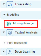
Moving Average is located under Forecasting ( ) in Modeling, on the left task pane. Use the drag-and-drop method to use the algorithm on the canvas. Click the algorithm to view and select different properties for analysis.
Refer to the Properties of Moving Average.
Consider a time-series data containing the following annual sales figures. We calculate the Moving Average over three years, for years 2015-2016-2017, 2016-2017-2018, and 2017-2018-2019. These values are given in the table below.
Year | Sales (In Millions) | Moving Average (Three Year Average) |
2015 | 5.0 | NA |
2016 | 5.4 | NA |
2017 | 5.7 | (5.0 + 5.4 + 5.7) / 3 = 5.366 |
2018 | 6.1 | (5.4 + 5.7 + 6.1) / 3 = 5.733 |
2019 | 6.4 | (5.7 + 6.1 + 6.4) / 3= 6.066 |
Properties of Moving Average
The available properties of Moving Average are as shown in the figure below.
The table below describes the different fields present on the properties of Moving Average.
Field | Description | Remark | |
| Run | It allows you to run the node. | - | |
| Explore | It allows you to explore the successfully executed node. | - | |
| Vertical Ellipses | The available options are
| - | |
Task Name | It is the name of the task selected on the workbook canvas. |
| |
Time ID Variable | It allows you to select the time variable. | The dataset should contain at least one time variable. | |
Target Variable | It allows you to select the variable for performing the moving Average. | The variable selected can be discrete or continuous. | |
Group By | It allows you to select the function for grouping identical data. |
| |
Advanced | Re-train | It allows you to select whether you want to re-train the moving average model. |
|
Interval | It allows you to select the interval on which you want to calculate the Moving Average. |
| |
Number of Periods for Forecasting | It allows you to select a specific number of periods you want to forecast based on the moving average results. |
| |
Confidence Level (%) | It allows you to select the confidence level with which we predict the results. |
| |
Window Size | It allows you to select the number of data points you want to select for calculating the Average. |
| |
Node Configuration | It allows you to select the instance of the Amazon Web Services (AWS) server to provide control on the execution of a task in a workbook or workflow. | For more details, refer to the Worker Node Configuration. | |
Example of Moving Average
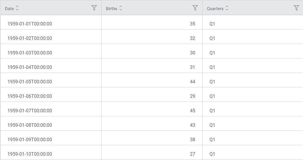
Consider a FemaleBirthData dataset with 365 records. It contains columns for Date, Number of Daily Births, and the corresponding Quarters. A snippet of the input data is shown in the figure given below.
We apply Moving Average on the input data. The selected values for Moving Average are given below.
Property | Value |
Time ID Variable | Date |
Target Variable | Births |
Group By | Quarter |
Retrain | Yes |
Interval | Day |
Number of Periods for Forecasting | 5 |
Confidence Level (%) | 95 |
Window Size | 4 |
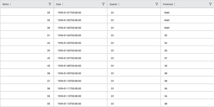
On the Data pane, you see the predicted values for the corresponding data points in the output. As you can see,
- Predicted values for the first three data points are 'NaN' since the selected window size is four (4).
- The Moving Average is calculated for subsequent subsets of four data points each. The resulting average is the predicted value for the fourth data point.
- The average of 35, 32, 30, and 31 is 32, the average of 32, 30, 31, and 44 is 34, and so on.
- Hence, the predicted number of births on 1959-01-04 is 32, against actual births (31). Also, the predicted number of births on 1959-01-05 is 34, as against forty-four (44) actual births.
Further, the Result page displays
- RMSE for actual and predicted values based on the calculated moving average
- The baseline and prediction plot for births, where the red curve indicates the variation in predicted births and the blue curve indicates the variation in actual births for the Quarter Q1.
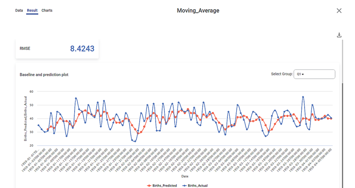
Similarly, you can change the Quarter from the Select Group field and obtain the corresponding plots.
Related Articles
ARIMA
ARIMA is located under Forecasting > Modeling > ARIMA. Use the drag-and-drop method (or double-click on the node) to use the algorithm in the canvas. Click the algorithm to view and select different properties for analysis. Properties of ARIMA The ...Components in Forecasting
Forecasting deals with the analysis and detection of trends in the time-series data. The components of forecasting are, Data Exploration: Data Exploration is used to explore the time-series data. It helps in identifying the underlying parameters ...Auto ARIMA
Auto ARIMA is located under Forecasting > Modeling > Auto ARIMA. Use the drag-and-drop method (or double-click on the node) to use the algorithm in the canvas. Click the algorithm to view and select different properties for analysis. Properties of ...Train Test Split
Train Test Split is located under Forecasting ( ) in Data Preparation, in the left task pane. Use the drag-and-drop method to use the algorithm in the canvas. Click the algorithm to view and select different properties for analysis. Refer to ...SARIMA
SARIMA is located under Forecasting( ) in Modeling, in the left task pane. Use the drag-and-drop method to use the algorithm in the canvas. Click the algorithm to view and select different properties for analysis. Refer to Properties of SARIMA. ARIMA ...