One Class SVM
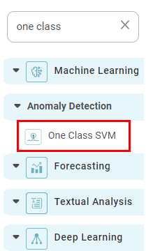
One Class SVM is located under Machine Learning ( ) in Anomaly Detection, in the left task pane. Use the drag-and-drop method to use the algorithm in the canvas. Click the algorithm to view and select different properties for analysis.
Refer to Properties of One-Class SVM.
Properties of One-Class SVM
The available properties of One-Class SVM are as shown below.
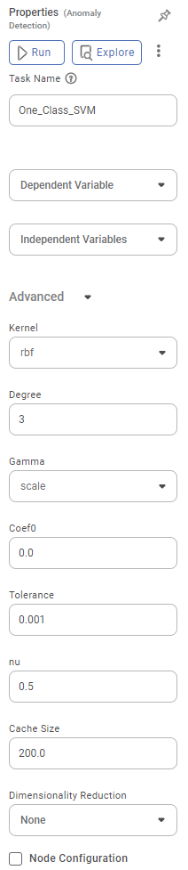
The table below describes the different fields on the properties of One-Class SVM.
Field | Description | Remark | |
|---|---|---|---|
| Run | It allows you to run the node | - | |
| Explore | It allows you to explore the successfully executed node. | - | |
| Vertical Ellipses | The available options are
| - | |
Task Name | It is the name of the task selected on the workbook canvas. |
| |
Dependent Variable | It allows you to select the dependent variable. |
| |
Independent Variable | It allows you to select Independent variables. |
| |
Advanced | Kernel | It allows you to select the kernel function to convert your data into a required form. |
|
Degree | It allows you to select the degree of the polynomial kernel function. |
| |
Gamma | It allows you to select the gamma parameter. |
| |
Coef0 | It is used to select the independent term for the kernel function. |
| |
Tolerance | It allows you to set the Tolerance value. |
| |
nu | It allows you to select the value of nu to limit the number of training errors. |
| |
Cache Size | It allows you to select the cache size. |
| |
Dimensionality Reduction | It allows you to select the dimensionality reduction technique. |
| |
Node Configuration | It allows you to select the instance of the AWS server to provide control over the execution of a task in a workbook or workflow. | For more details, refer to Worker Node Configuration. | |
Example of One-Class SVM
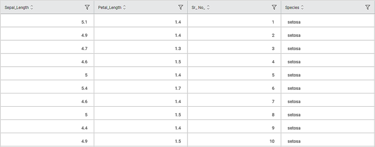
Consider an Iris dataset with two classes of species, Iris-setosa and Iris-versicolor. A snippet of the input data is shown below.
Scenario 1:
We apply One-Class SVM to the input data by selecting the Species column as the Dependent Variable. The selected values are given below.
Property | Value |
Dependent Variable | Species |
Independent Variable | Sepal Length, Sepal Width, Petal Length, Petal Width |
Kernel | rbf |
Degree | 3 |
Gamma | scale |
Coef0 | 0.0 |
Tolerance | 0.001 |
Nu | 0.5 |
Cache Size | 200.0 |
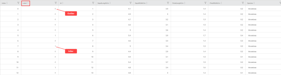
In the Data tab, you see a categorical Label column added to the original data. The Label values decide whether the selected value is Inlier or Outlier.
- Label = 1 for an Inlier (represented in Blue in Rubiscape)
- Label = -1 for an Outlier (represented in Red in Rubiscape)
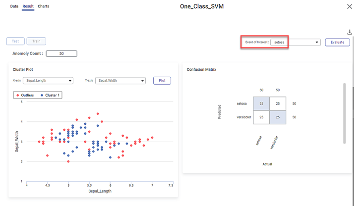
- The following KPIs for the selected event of interest, that is, species
- In this case, the event of interest is Iris-setosa
- Cluster Plot between two independent variables.
- In this case, it is plotted between Sepal Length and Sepal Width
- The blue dots represent the inliers, the data points belonging to the distribution. Here, all the blue dots belong to Cluster 1.
- The red dots represent the outliers, that is, the data points not belonging to the distribution
- You can change the independent variables and observe the cluster plots for different combinations of independent variables
- Make sure to select different variables for the cluster plot. If you select the same variable, you see the error message 'Please select different x-axis and y-axis labels.'
- Confusion Matrix between the predicted and actual values of the two species.
- The shaded diagonal cells show the correctly predicted categories. For example, 14 data points out of 50 for Iris-setosa species are correctly predicted.
- The remaining cells indicate the wrongly predicted categories, that is, errors.
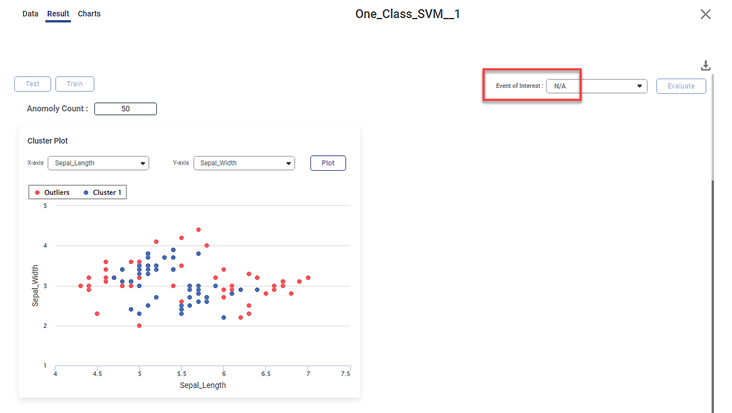
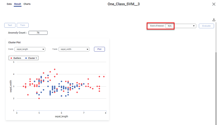
Scenario 2:
We apply One-Class SVM to the input data. However, now we do not select any variable as a dependent variable. The other selected values remain the same.
On the result page, you observe the cluster plot. The KPIs and Confusion Matrix are not displayed since there is no event of interest option.
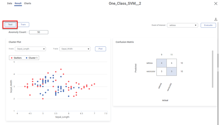
Scenario 3:
We apply the train-test split to the above dataset before applying One-Class SVM.
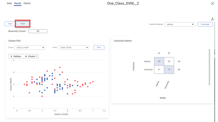
Various KPIs and Confusion Matrix for Test and Train datasets are different when you explore the results. However, the cluster plot remains the same since it is plotted for the entire dataset.
For example, the figure below displays the result page for the Test dataset.
The figure below displays the result page for the Train dataset.
Scenario 4:
We use a different dataset containing more than two classes. For example, we take an Iris dataset with three classes of species, Iris-setosa, Iris-versicolor, and Iris-virginica.
In this case, run the One-Class SVM algorithm with Species as the dependent variable. When you explore the results, the cluster plot is displayed. However, there is no list of species available in the event of interest field. Hence, KPIs and Confusion Matrix are not displayed.
Related Articles
One Sample Z Test
One sample Z Test is located under Model Studio > Statistical Analysis > One Sample z-test on the left task pane. Use the drag-and-drop method (or double-click on the node) to use the algorithm in the canvas. Click the algorithm to view and select ...One Way ANOVA
One Way ANOVA is located under Model Studio ( ) in ANOVA Analysis under Statistical Analysis, in the task pane on the left. Use the drag-and-drop method to use the algorithm in the canvas. Click the algorithm to view and select different properties ...One Sample T Test
One Sample t Test is located under Model Studio > Statistical Analysis > One sample t Test. Use the drag-and-drop method (or double-click on the node) to use the algorithm in the canvas. Then, Click the algorithm to view and select different ...One Sample Proportion Test
One Sample Proportion Test is located under Model Studio in Statistical Analysis below Hypothesis Test, Parametric Test in the left task pane. Use the drag-and-drop method or double-click to use the algorithm in the canvas. Click the algorithm to ...One Sample Wilcoxon Signed Rank Test
One Sample Wilcoxon Signed Rank Test is located under Model Studio () in Statistical Analysis below Hypothesis Test, under Non-Parametric Test in the left task pane. Use the drag-and-drop method or double-click to use the algorithm in the canvas. ...