Random Forest
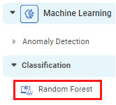
Random Forest is located under Machine Learning (  ) in Classification, in the left task pane. Use the drag-and-drop method (or double-click on the node) to use the algorithm in the canvas. Click the algorithm to view and select different properties for analysis.
Refer to Properties of Random Forest.
Properties of Random Forest
The available properties of the Random Forest are as shown in the figure below.
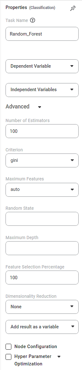
The table given below describes the different fields present on the properties pane of Random Forest.
Field | Description | Remark |
|---|---|---|
| Run | It allows you to run the node | - |
| Explore | It allows you to explore the successfully executed node. | - |
| Vertical Ellipses | The available options are
| - |
Task Name | It is the name of the task selected on the workbook canvas. | You can click the text field to edit or modify the task's name. |
Dependent Variable | It allows you to select the dependent variable. |
|
Independent variables | It allows you to select the experimental or predictor variable(s). |
|
Advanced | ||
Number of Estimators | It allows you to select the number of base estimators in the ensemble. |
|
Criterion | It allows you to select the Decision-making criterion to be used. |
|
Maximum Features | It allows you to select the maximum number of features to be considered for the best split. |
|
Random State | It allows you to select a random combination of train and test for the classifier. |
|
Maximum Depth | It allows you to set the length of the decision tree. |
|
Feature Selection Percentage | It is used to decide the feature importance of the selected variable. |
|
Dimensionality Reduction | It allows you to select the dimensionality reduction technique. |
|
Add Result as a Variable | It allows you to select any of the result parameters as the variable. |
|
Node Configuration | It allows you to select the instance of the AWS server to provide control on the execution of a task in a workbook or workflow. | For more details, refer to Worker Node Configuration. |
Hyperparameter Optimization | It allows you to select parameters for Hyperparameter Optimization. | For more details, refer to Hyperparameter Optimization. |
Example of Random Forest
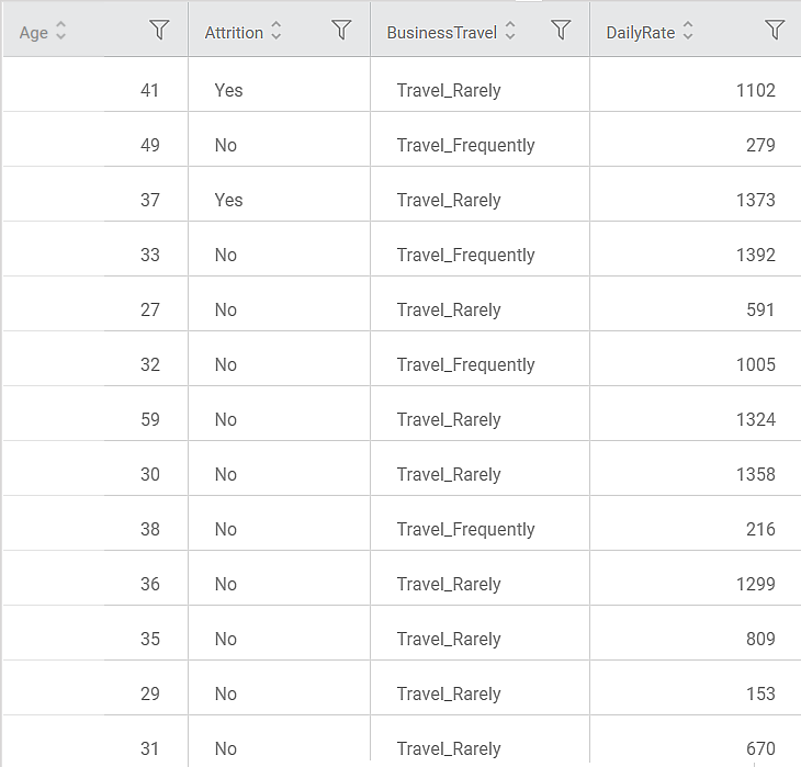
Consider an HR dataset with over 1400 rows and 30 columns. There are multiple features like Attrition, BusinessTravel, DailyRate, PercentSalaryHike, PerformanceRating, and so on in the dataset. The dataset can study the impact of multiple factors on employee attrition.
A snippet of input data is shown in the figure given below.
In the Properties pane, the following values are selected.
Property | Value |
|---|---|
Dependent Variable | Attrition |
Independent Variables | Age, DailyRate, Education, JobSatisfaction, PercentSalaryHike, StockOptionLevel, WorkLifeBalance |
No. of Estimators | 100 |
Criterion | gini |
Maximum Features | auto |
Random State | 3 |
Maximum Depth | 10 |
Feature Selection Percentage | 60 |
Dimensionality Reduction | None |
Add result as a variable | Accuracy, Sensitivity, Specificity, FScore |
Notes: |
|
Since we select Accuracy, Sensitivity, Specificity, and FScore as the performance metrics, the following variables are created corresponding to the two Events of Interest, "Yes" and "No.". The value of accuracy remains same for both the events. Thus, you have eight 7 new variables created.
For example, Random_Forest_Accuracy_No, and Random_Forest_Accuracy_Yes are the variables created corresponding to the Accuracy metric for the events "Yes" and "No."
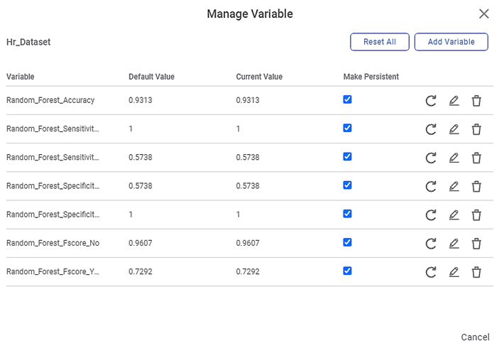
Note: | As you can see, the Default and Current values for each variable are the same, and they are also the values for the performance metrics displayed on the Result page. |
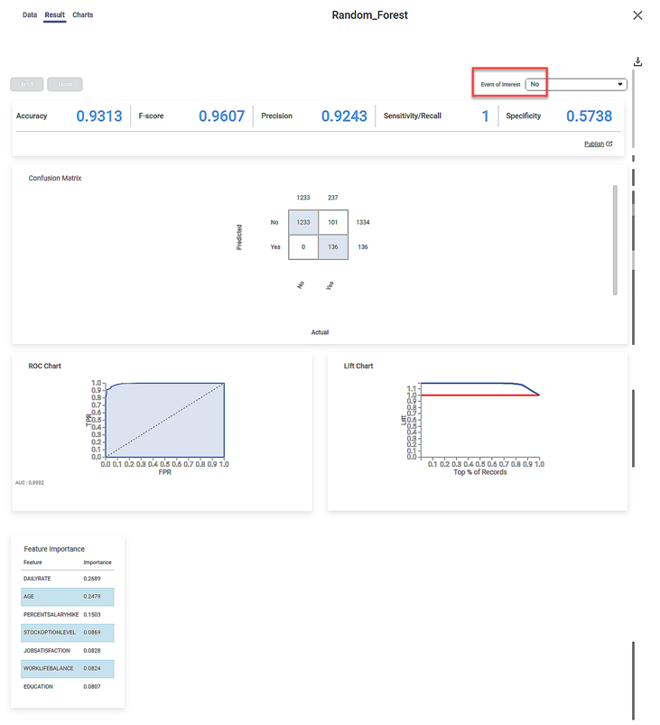
The Result Page for the Event of Interest "No" is shown below.
The Result page for the Event of Interest "Yes" is shown below.
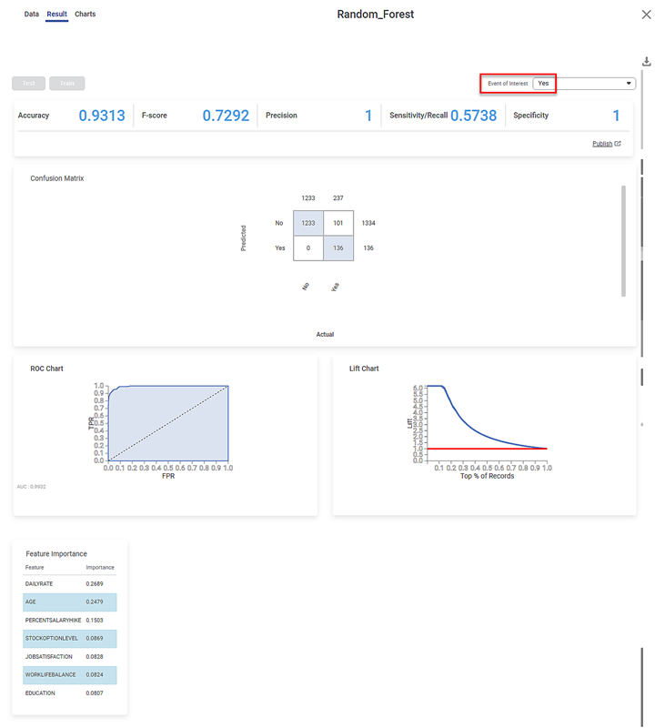
The Result page displays
- The performance metrics Accuracy, FScore, Sensitivity, and Specificity, for the two events of interest.
- You can see that the accuracy for the two events is constant at 0.9313.
- The three remaining metrics have different values for the two events.
- The Confusion Matrix for the predicted and actual values of the two Events of Interest.
- The shaded diagonal cells show the correctly predicted categories. For example, 1233 "No" and 136 "Yes" Attrition values are correctly predicted.
- The remaining cells indicate the wrongly predicted categories. For example, 101 "Yes" Attrition values are wrongly predicted as "No."
- The Receiver Operating Characteristics (ROC) charts for the two Events of Interest.
- You can see that the ROC curve is identical for both events.
- The Area Under Curve (AUC) for the ROC chart is 0.9906.
- Since the value is high (close to 1), the Random Forest model is meaningful and clearly distinguishes between the two classes or events of interest (of Attrition).
- The Lift Charts for the two Events of Interest.
- You can see that the Lift Charts are different for the two events
- The area of the region between the life curve (blue) and baseline (red) is different for the two events.
- Since the area for the Event of Interest "Yes" is more, we can conclude that the Random Forest algorithm more clearly classifies this event.
- The Feature Importance of the selected independent variables.
- The feature importance is expressed as a decimal number
- The features are arranged in descending order of their importance.
- Thus, DailyRate is most important while WorkLifeBalance is the least important feature for deciding employee attrition.
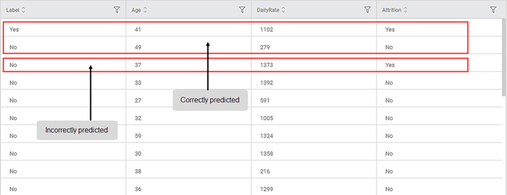
The Data page displays
- One additional Label column Two columns: Index and Label. Since the image for the Data tab does not show the index column, should we still add it? No.
- The dependent variable column (Attrition)
- The maximum importance features, that is, features for which the sum of feature importance is less than or equal to 0.6 (Age and DailyRate)
- You can compare the corresponding values in the Label and Attrition columns and observe the correctly and incorrectly predicted values
Related Articles
Random Forest Regression
Random Forest Regression is located under Machine Learning ( ) > Regression > Random Forest Regression Use the drag-and-drop method (or double-click on the node) to use the algorithm in the canvas. Click the algorithm to view and select different ...Isolation Forest
Isolation Forest is located under Machine Learning () in Anomaly Detection, in the left task pane. Use the drag-and-drop method (or double-click on the node) to use the algorithm in the canvas. Click the algorithm to view and select different ...Classification
Notes: The Reader (Dataset) should be connected to the algorithm. Missing values should not be present in any rows or columns of the reader. To find out missing values in a data, use Descriptive Statistics. Refer to Descriptive Statistics. If missing ...Task Wise GPU Integration for Machine Learning Algorithms.
Overview GPU execution support has been introduced for supported Machine Learning algorithms to improve processing performance, execution efficiency, and scalability for machine learning workloads. Users can now enable GPU execution at task level for ...MLOPS - Machine Learning Operations
Introduction: Why Rubiscape MLOps? Rubiscape MLOps provides an end-to-end environment for building, tracking, publishing, and serving machine learning models. It ensures experiment reproducibility, streamlined deployment, and centralized model ...