Linear Regression
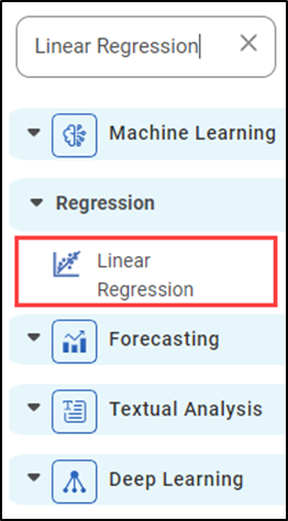
Linear Regression is located under Machine Learning (  ) in Regression, in the task pane on the left. Use the drag-and-drop method to use the algorithm in the canvas. Click the algorithm to view and select different properties for analysis. Refer to Properties of Linear Regression.
Properties of Linear Regression
The available properties of Linear Regression are shown in the figure below.
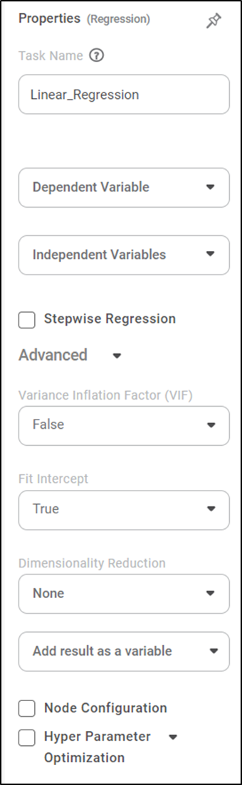
The table below describes the different fields present in the properties of Linear Regression.
Field | Description | Remark | |
|---|---|---|---|
| Run | It allows you to run the node. | - | |
| Explore | It allows you to explore the successfully executed node. | - | |
| Vertical Ellipses | The available options are
| - | |
Task Name | It displays the name of the selected task. | You can click the text field to edit or modify the task's name as required. | |
Dependent Variable | It allows you to select the variable from the drop-down list for which we need to predict the values of the dependent variable y. |
| |
Independent Variables | It allows you to select the experimental or predictor variable(s) x. |
| |
Stepwise Regression | It allows the user to select methods of stepwise regression. |
| |
Advanced | Variance Inflation Factor | It allows you to detect multicollinearity in regression analysis. |
|
Fit | It allows you to select whether you want to calculate the value of constant (c) for your model. |
| |
Dimensionality |
|
| |
Add Result as a variable | It allows you to select whether the result of the algorithm is to be added as a variable. | For more details, refer to Adding Result as a Variable. | |
Node Configuration | It allows you to select the instance of the AWS server to provide control over the execution of a task in a workbook or workflow. | For more details, refer to Worker Node Configuration | |
Hyper Parameter Optimization | It allows you to select parameters for optimization. | For more details, refer to Hyper parameter Optimization | |
Stepwise Regression Methods
You can choose either of the following iterative regression methods in Machine Learning.
- Forward Selection
- It starts with no variable in the model.
- The system adds one variable in the model and checks whether the model is statistically significant.
- If the model is statistically significant then the variable is added to the model.
- The above steps are repeated till the system gets optimal results.
- Backward Elimination
- It starts with a set of independent variables.
- The system removes one variable from the model.
- Then checks whether the model is statistically significant. If the model is not statistically significant then the variable is removed from the model.
- The above steps are repeated till the system gets optimal results.
- Bidirectional Selection
- It is a combination of the Forward selection and Backward elimination methods.
- It adds and removes the independent variable combinations. Checks if the model is statistically significant.
- Repeat the steps till it gets all the independent variables between the significant level.
Example of Linear Regression
The Linear Regression is applied to a Used credit card dataset in the example below. We select Income, Limit, Cards, Education, Age, and Balance as the independent variables and Rating as the dependent variable. The result of the XGBoost Regression is displayed in the figure below.
The Result page of Linear Regression is shown below.
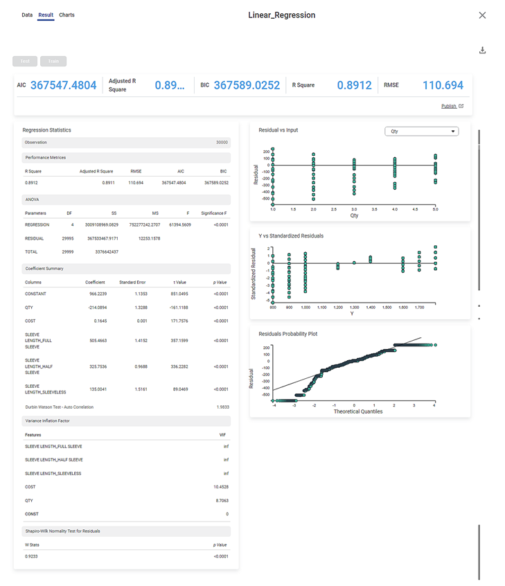
The result page is segregated into the following sections.
- Key Performance Indicator (KPI)
- Regression Statistics
- Graphical representation
Section 1: Key Performance Indicator (KPI)
The figure below displays various KPIs calculated in Linear Regression.

The table below describes multiple (KPIs) on the result page.
Performance Metric | Description | Remark |
|---|---|---|
RMSE (Root Mean Squared Error) | It is the square root of the averaged squared difference between the actual values and the predicted values. | It is the most commonly used performance metric of the model. |
R Square | It is the statistical measure that determines the proportion of variance in the dependent variable that is explained by the independent variables. | Value is always between 0 and 1. |
Adjusted R Square | It is an improvement of R Square. It adjusts for the increasing predictors and only shows improvement if there is a real improvement. | Adjusted R Square is always lower than R Square. |
AIC (Akaike Information Criterion) | AIC is an estimator of errors in predicted values and signifies the quality of the model for a given dataset. | A model with the least AIC is preferred. |
BIC | BIC is a criterion for model selection amongst a finite set of models. | A model with the least BIC is preferred. |
| MSE (Mean Squared Error) | It is the averaged squared difference between the actual values and the predicted values. | A model with low MSE is preferred. |
| MAE (Mean Absolute Error) | It the absolute value of difference between actual and predicted values | A model with low MAE is preferred. |
| MAPE ( Mean Absolute Percentage Error) | it is the average magnitude of error produced by a model, or how far off predictions are on average. | A model with low MAPE is preferred |
Section 2: Regression Statistics
Regression Statistics consists of ANOVA, Performance Metrices, Coefficient Summary, Durbin Watson Test - Auto Correlation, Variance Inflation Factor, and Shapiro-Wilk Normality Test for Residuals for each of the selected independent (predictor) variables.
The Observation displays the total number of rows considered in Linear Regression.

The Performance Metrices consist of all KPI Details.
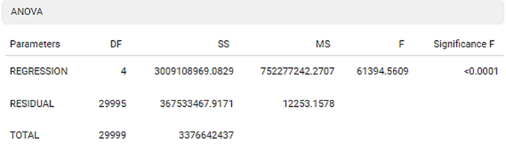
The ANOVA test calculates the difference in independent variable means. It helps you distinguish the difference in the behavior of the independent variable. To know more about ANOVA, click here.
You see values like Degrees of Freedom (DF), Sum of Squares (SS), Mean Sum of Squares (MS), F statistic of ANOVA, and Significance F.
DF represents The number of independent values that can differ freely within the constraints imposed on them.
SS is the sum of the square of the variations. Variation is the difference (or spread) of each value from the mean.
MS is the value obtained by dividing the Sum of Squares by Degrees of Freedom
F statistic of ANOVA indicates whether the regression model provides a better fit than a model without independent variables.
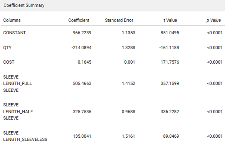
The Coefficient Summary displays the coefficient correlation between a dependent variable and each independent variable. If the coefficient of correlation is less than zero then there is a negative correlation between the dependent and an independent variable. In this example, there is a negative correlation between Age and KM.
It also calculates the p value based on the t statistic. The null hypothesis is rejected if the p value is less than level of significance (alpha). In the given example, the p value is less than level of significance (alpha).
The Durbin Watson Test determines autocorrelation between the residuals. If the test value is less than 2 then there is a positive correlation in the sample.
To find out more details about the Durbin Watson test, Click here

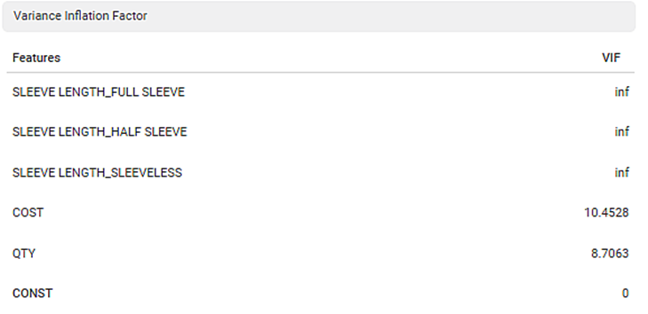
The Variance Inflation Factor is used to detect multicollinearity in regression analysis. VIF is calculated by selecting one predictor and regressing it against all other predictors in the model.
The value of VIF is equal to or greater than 1. If VIF = 1, the predictors are not correlated. If VIF is between 1 and 5, they are moderately correlated. For any value greater than 5, the predictors are heavily correlated. The higher the value of VIF, the lower the reliability of the regression results, and ultimately the model.
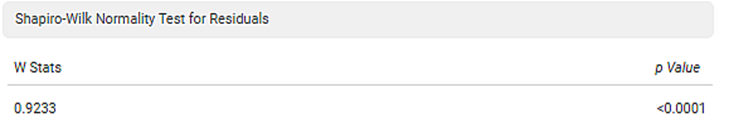
The Shapiro-Wilk Normality Test for Residuals test checks if the input data comes from a normal distribution. If the p value is less than 0.05 then reject the null hypothesis. In the given example, the p value is less than 0.05; hence the null hypothesis is rejected. To find out more details about Shapiro-Wilk Normality Test, Click here
Section 3: Graphical representation
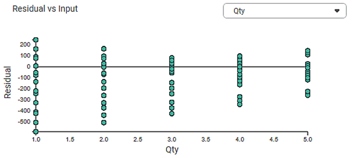
1. Residual vs. Input graph:
- If this graph creates a pattern, then the sample is improper.
- The graph is plotted with the Independent variable on the x-axis and Residual points on the y-axis.
- On the right side, there is an independent variable dropdown. In this example, independent variables like Age, KM, HP, and CC appear in the dropdown.
- The input variable is the same as in the dropdown. In the figure below, the input variable is Age, the same as in the dropdown.
- If this graph follows a pattern then the data is not normally distributed.
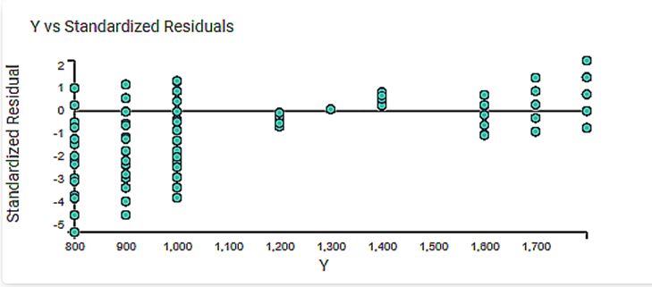
2. The Y vs. Standardized Residuals graph plots the dependent variable, Price, on the x-axis and the Standardized Residual on the y-axis.
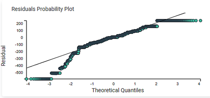
3. The Residuals Probability Plots the Independent variable on the x-axis and standardized Residuals on the y-axis. It helps to identify whether the error terms are normally distributed.
4. The Best Features displays the order of the Independent variable that provides the best result of R2. You have performed linear regression with the backward compatibility method in this example. The best sequence of the independent variable is Age, KM, HP, and CC. This order is based on the adjusted R2.
Related Articles
Binomial Logistic Regression
Binomial Logistic Regression is located under Machine Learning () in Data Classification, in the task pane on the left. Use drag-and-drop method to use the algorithm in the canvas. Click the algorithm to view and select different properties for ...MLP Neural Network in Regression
The MLP Neural Network is located under Machine Learning in Regression, on the left task pane. Alternatively, use the search bar for finding the MLP Neural Network algorithm. Use the drag-and-drop method or double-click to use the algorithm in the ...Coefficient Summary
Overview Rubiscape now provides Coefficient Summary support for Ridge, Lasso, and Poisson regression, extending the existing functionality available for Linear and Polynomial Regression. This ensures all supported regression models display their ...Poisson Regression
Poisson Regression is located under Machine Learning () under Regression, in the left task pane. Use the drag-and-drop method to use the algorithm in the canvas. Click the algorithm to view and select different properties for analysis. Refer to ...Polynomial Regression
Polynomial Regression is located under Machine Learning () under Regression, in the left task pane. Use the drag-and-drop method to use the algorithm in the canvas. Click the algorithm to view and select different properties for analysis. Refer to ...