Extreme Gradient Boost Classification (XGBoost)
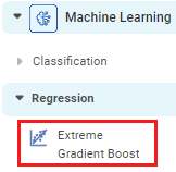
Extreme Gradient Boost is located under Machine Learning ( ) in Classification, in the task pane on the left. Use the drag-and-drop method (or double-click on the node) to use the algorithm in the canvas. Click the algorithm to view and select different properties for analysis.
Refer to Properties of Extreme Gradient Boost.
Properties of Extreme Gradient Boost
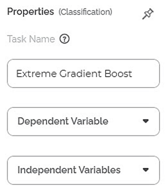
The total available properties of the XGBoost classifier are as shown in Properties and Advance Properties figures given below.
The advanced properties of XGBoost classifier are as shown in the figure given below.
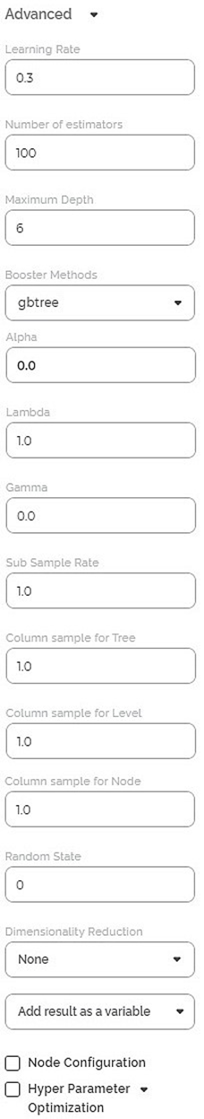
The table below describes the different fields present on the Properties pane of the XGBoost Classifier, including the basic and advanced properties.
Field | Description | Remark | |
| Run | It allows you to run the node. | - | |
| Explore | It allows you to explore the successfully executed node. | - | |
| Vertical Ellipses | The available options are
| - | |
Task Name | It displays the name of the selected task. | You can click the text field to edit or modify the name of the task as required. | |
Dependent Variable | It allows you to select the variable for which you want to perform the task. |
| |
Independent Variables | It allows you to select the experimental or predictor variable(s). |
| |
Advanced | Learning Rate | It allows you to set the weight applied to each classifier during each boosting iteration. | The higher learning rate results in an increased contribution of each classifier. |
Number of estimators | It allows you to enter the number of estimators. Estimator stands for Trees. It takes the input from the user for the number of trees to build the ensemble model. |
| |
Maximum Depth | It allows you to set the depth of the Decision Tree.
|
| |
Booster Method | It allows you to select the booster to use at each iteration. | The available options are,
gbtree and dart are optimization methods used for classification problems, whereas; the gblinear method is used for a regression problem. | |
Alpha | It allows you to enter a constant that multiplies the L1 term. | The default value is 1.0. | |
Lambda | It allows you to enter a constant that multiplies the L2 term. | The default value is 1.0. | |
Gamma | It allows you to enter the minimum loss reduction required to make a further partition on a leaf node of the tree. |
| |
Sub Sample Rate | It allows you to enter the fraction of observations to be randomly sampled for each tree. |
| |
Column Sample for Tree | It allows you to enter the subsample ratio of columns when constructing each tree. |
| |
Column Sample for Level | It allows you to enter the subsample ratio of columns for each level. |
| |
Column Sample for Node | It allows you to enter the subsample ratio of columns for each node, i.e., split. |
| |
Random state | It allows you to enter the random state value |
| |
Dimensionality Reduction | It allows you to select the dimensionality reduction technique. |
| |
Node Configuration | It allows you to select the instance of the AWS server to provide control on the execution of a task in a workbook or workflow. | For more details, refer to Worker Node Configuration. | |
| Hyperparameter Optimization | It allows you to select parameters for Hyperparameter Optimization. | For more details, refer to Hyperparameter Optimization. |
Example of Extreme Gradient boost
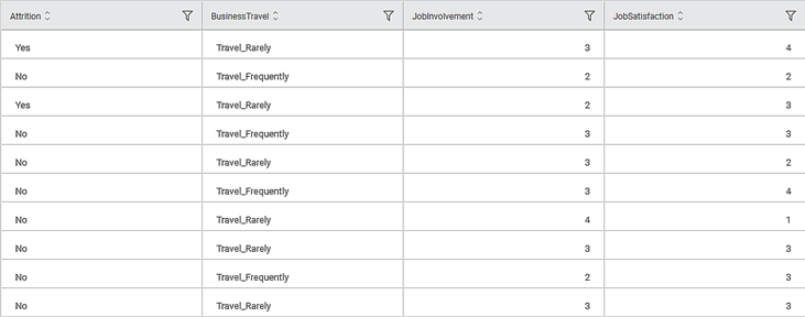
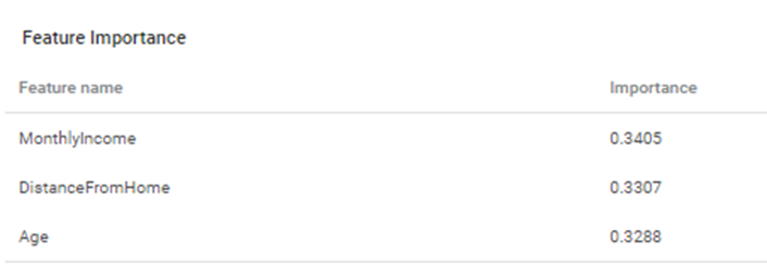
Consider an HR dataset that contains various parameters. Here, three parameters - Age, Distance from home, and Monthly Income are selected to perform the attrition analysis. The intention is to study the impact of these parameters on the attrition of employees. We analyze which factors have the most influence on the attrition of employees in an organization.
A snippet of input data is shown in the figure given below.
The selected values for properties of the XGBoost classifier are given in the table below.
Property | Value |
Dependent Variable | Attrition |
Independent Variables | Age, Distance from home, and Monthly Income |
Learning Rate | 0.3 |
Number of estimators | 100 |
Maximum Depth | 6 |
Booster Method | gbtree |
Alpha | 0.0 |
Lambda | 1.0 |
Gamma | 0.0 |
Sub Sample Rate | 1.0 |
Column Sample for Tree | 1.0 |
Column Sample for Level | 1.0 |
Column Sample for Node | 1.0 |
Random state | 0 |
Dimensionality Reduction | None |
Node Configuration | None |
Hyperparameter Optimization | None |
XGBoost Classifier gives results for Train as well as Test data.

The table given below describes the various Key Parameters for Train Data present in the result.
Field | Description | Remark |
Sensitivity | It gives the ability of a test to identify the positive results correctly. |
|
Specificity | It gives the ratio of the correctly classified negative samples to the total number of negative samples. |
|
F-score |
|
|
Accuracy | Accuracy is the ratio of the total number of correct predictions made by the model to the total predictions. |
|
| Precision | Precision is the ratio of the True positive to the sum of True positive and False Positive. It represents positive predicted values by the model |
|
The Confusion Matrix obtained for the XGBoost Classifier is given below.
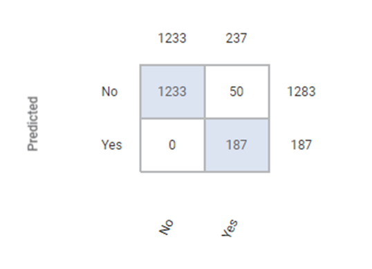
The table below describes the various values present in the Confusion Matrix.
Field | Description | Remark |
True Positive (TP) | It gives an outcome where the model correctly predicts the positive class. | Here, the true positive count is 187. |
True Negative(TN) | It gives an outcome where the model correctly predicts the negative class. | Here, the true negative count is 1233. |
False Positive (FP) |
| Here, the false positive count is 0. |
False Negative(FN) |
| Here, the false negative count is 50. |
Note: | The model that has minimum Type 1 and Type 2 errors is the best fit model. |
The ROC and Lift charts for the XGBoost Classifier are given below.
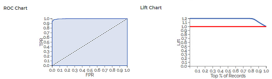
The table given below describes the ROC Chart and the Lift Curve
Field | Description | Remark |
ROC Chart | The Receiver Operating Curve (ROC) is a probability curve that helps measure the performance of a classification model at various threshold settings.
|
|
Lift Chart |
|
|
Related Articles
Extreme Gradient Boost Regression (XGBoost)
XGBoost Regression is located under Machine Learning ( ) in Regression, in the left task pane. Use the drag-and-drop method to use the algorithm in the canvas. Click the algorithm to view and select different properties for analysis. Refer to ...Classification
Notes: The Reader (Dataset) should be connected to the algorithm. Missing values should not be present in any rows or columns of the reader. To find out missing values in a data, use Descriptive Statistics. Refer to Descriptive Statistics. If missing ...Gradient Boosting in Classification
The category Gradient Boosting is located under Machine Learning in Classification on the feature studio. Alternatively, use the search bar to find the Gradient Boosting test feature. Use the drag-and-drop method or double-click to use the algorithm ...AdaBoost in Classification
You can find AdaBoost under the Machine Learning section in the Classification category on Feature Studio. Alternatively, use the search bar to find the AdaBoost algorithm. Use the drag-and-drop method or double-click to use the algorithm in the ...Task Wise GPU Integration for Machine Learning Algorithms.
Overview GPU execution support has been introduced for supported Machine Learning algorithms to improve processing performance, execution efficiency, and scalability for machine learning workloads. Users can now enable GPU execution at task level for ...